Particula tour

We have designed particula around object-oriented programming principles where physics entities inherit from each other.

1. It all starts with an Environment object (class) where temperature, pressure, and other derived properties are defined. For now, the two main derived properties are the dynamic viscosity and mean free path.

2. Then, the Vapor object inherits from Environment and adds its own properties, mainly vapor properties like radius and density, but also derived properties like the driving force of condensation.

3. The most involved object Particle builds on Vapor (and thus Environment). It is split into steps to isolate different components (e.g. making a distribution, making particle instances, calculating condensation, and calculating coagulation are all split into different objects that build on each other). In Particle, the idea is to form a fully equipped particle distribution, whose properties are readily available and calculated.

4. Up to Particle, there is no sense of a time dimension. To add one, we create the Rates object who takes as input the Particle object, thus explicitly allowing dynamics-specific calculations, or “rates”.

5. Finally, a dynamic Solver object builds on Rates and propagates the Particle object in time.

Setup

Let’s first get the needed packages and set up our computational environment.

try:
    import particula, matplotlib
except ImportError:
    print("Setting up computational environment...")
    %pip install -U particula -qqq
    %pip install matplotlib -qqq

from particula.particle import Particle
from particula.rates import Rates
from matplotlib import pyplot as plt
import numpy as np

Defining a distribution

Defining a distribution in particula is easy! Simply import the Particle class and pass some keyword arguments to it. Here we interested in a bimodal particle distribution, with different modes and different geometric standard deviations (gsigma) and different amplitude (particle_number). While at it, we might as well calculate rates and disabling the lazy execution so that we do not recalculate the rates at every call.

deets = {
    "mode": [10e-9, 70e-9],
    "gsigma": [1.6, 2.0],
    "nbins": 4000,
    "particle_number": [17/20, 3/20],
}
part_dist = Particle(**deets)
r = Rates(particle=part_dist, lazy=False)

We define a simple plot utility to plot some of the properties of this distribution.

def plot_some(x, y, grid="semilogx", title=None, label=None):
    """ plot y vs x with grid, providing title and label """
    if grid == "loglog":
        plt.loglog(x.m, y.m, label=label)
    else:
        plt.semilogx(x.m, y.m, label=label);
    if label is not None:
        plt.legend()
    plt.title(title)
    plt.xlabel(f"{x.u}"); plt.ylabel(f"{y.u}");

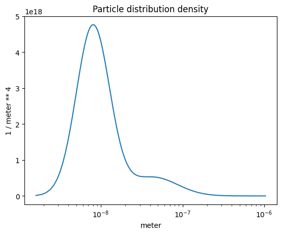
Particle number concentration density

One way to think about this is to integrate the curve, that yields exactly 1e5 /cc which is the total number concentration. Try it! (Copy the code block below and execute it after or before the next cell.)

np.trapz(part_dist.particle_distribution(), part_dist.particle_radius)

plot_some(
    x=part_dist.particle_radius,
    y=part_dist.particle_distribution(),
    title="Particle distribution density",
)

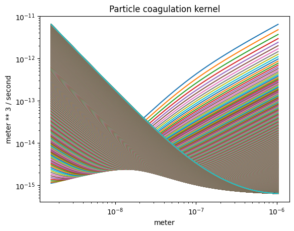
The coagulation kernel

plot_some(
    x=part_dist.particle_radius,
    y=part_dist.coagulation(),
    title="Particle coagulation kernel",
    grid="loglog"
)

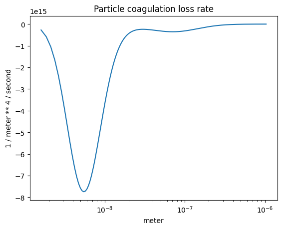
The coagulation loss rate

plot_some(
    x=part_dist.particle_radius,
    y=-r.coagulation_loss(),
    title="Particle coagulation loss rate",
)

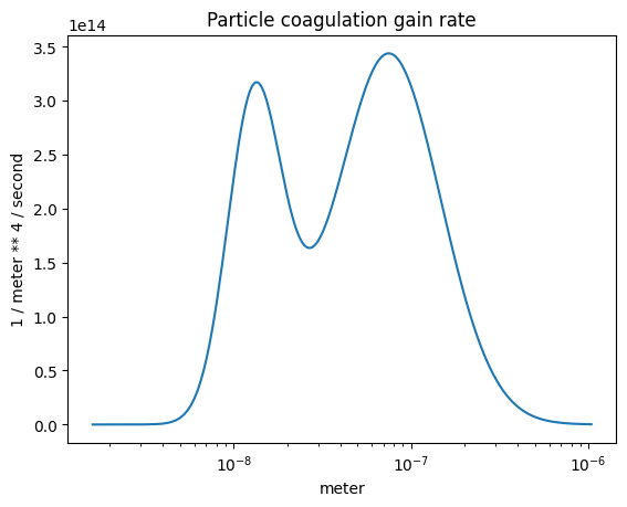
The coagulation gain rate

plot_some(
    x=part_dist.particle_radius,
    y=r.coagulation_gain(),
    title="Particle coagulation gain rate",
)

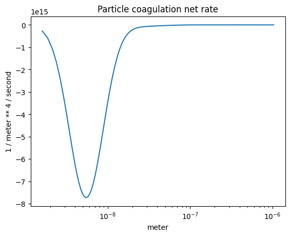
The coagulation net rate

plot_some(
    x=part_dist.particle_radius,
    y=r.coagulation_rate(),
    title="Particle coagulation net rate",
)

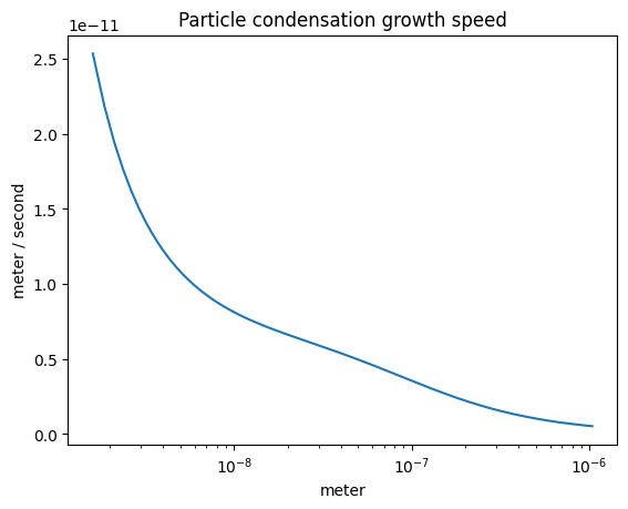
The condensation growth speed

plot_some(
    x=part_dist.particle_radius,
    y=r.condensation_growth_speed(),
    title="Particle condensation growth speed",
)

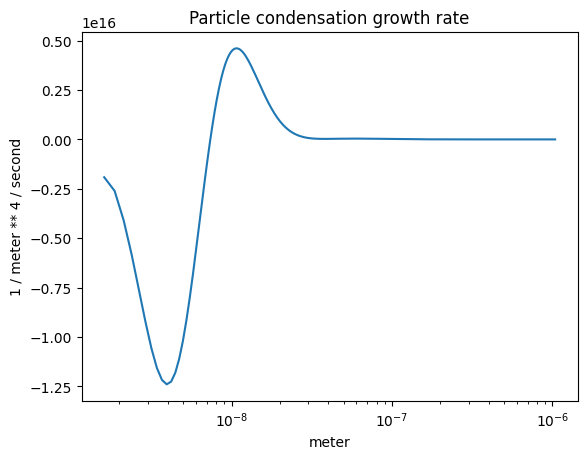
The condensation growth rate

plot_some(
    x=part_dist.particle_radius,
    y=r.condensation_growth_rate(),
    title="Particle condensation growth rate",
)

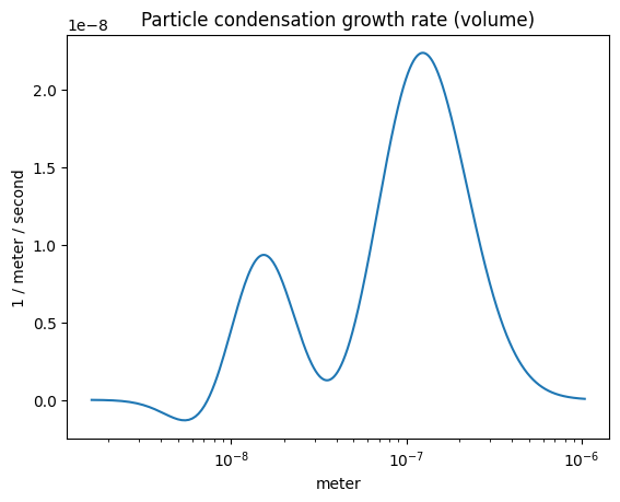
The condensation growth rate (volume-wise)

plot_some(
    x=part_dist.particle_radius,
    y=r.condensation_growth_rate()*part_dist.particle_radius**3,
    title="Particle condensation growth rate (volume)",
)

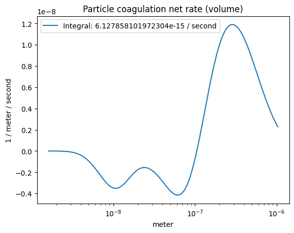
The coagulation net rate (volume-wise)

Note the integration yields a small number, meaning the mass is conserved!

plot_some(
    x=part_dist.particle_radius,
    y=r.coagulation_rate()*part_dist.particle_radius**3,
    title="Particle coagulation net rate (volume)",
    label=f"Integral: {np.trapz(r.coagulation_rate()*part_dist.particle_radius**3, part_dist.particle_radius)}"
)

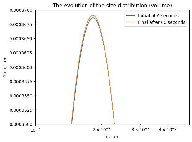
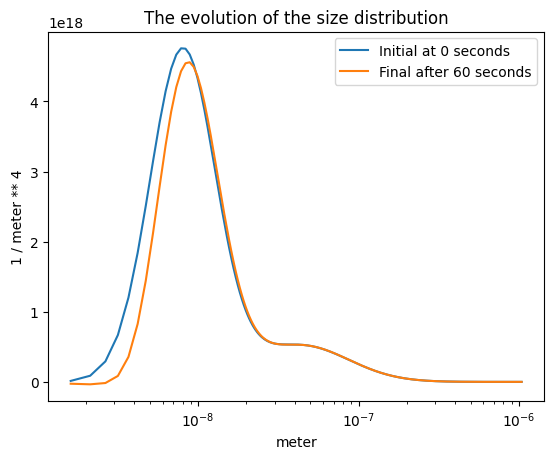
A solver

If you are adventurous, you can even propagate the define distribution in time! We use a rather simple solver here, but it still takes time as it has to recalculate all the rates at every time step. We reduce the nbins to make it slightly faster, but it may not even run on a super tiny (free) machine.

from particula.dynamics import Solver
deets = {
    "mode": [10e-9, 70e-9],
    "gsigma": [1.6, 2.0],
    "nbins": 2000,
    "particle_number": [17/20, 3/20],
}
part_dist = Particle(**deets)
r = Rates(particle=part_dist, lazy=True)
time_span = [0, 60]
s = Solver(particle=part_dist, time_span=time_span)
sols = s.solution()
plt.semilogx(part_dist.particle_radius.m, sols[0].m, label=f"Initial at {time_span[0]} seconds")
plt.semilogx(part_dist.particle_radius.m, sols[-1].m, label=f"Final after {time_span[-1]} seconds")
plt.xlabel(f"{part_dist.particle_radius.u}")
plt.ylabel(f"{sols[0].u}")
plt.title("The evolution of the size distribution")
plt.legend();

plt.semilogx(
    part_dist.particle_radius.m,
    sols[0].m*part_dist.particle_radius.m**3,
    label=f"Initial at {time_span[0]} seconds"
)
plt.semilogx(
    part_dist.particle_radius.m,
    sols[-1].m*part_dist.particle_radius.m**3,
    label=f"Final after {time_span[-1]} seconds"
)
plt.legend()
plt.xlabel(f"{part_dist.particle_radius.u}")
plt.ylabel(f"{sols[0].u*part_dist.particle_radius.u**3}")
plt.title("The evolution of the size distribution (volume)")
plt.xlim([1e-7, 5e-7]); plt.ylim([35e-5, 37e-5]);