

Run, save and resume a closed aerosol growth experiment
Run, save and resume a closed aerosol growth experiment
Section titled “Run, save and resume a closed aerosol growth experiment”How much does a finite vapor reservoir grow an initially monodisperse aerosol? We follow 100 nm organic particles for ten minutes, save their history, restart halfway through, and repeat with twice the initial vapor. The inputs are an illustrative low-volatility organic case, not a fit to a particular compound or chamber measurement. All calculation runs on native NumPy CPU arrays.
Initial number density is 1000 cm⁻³ (10⁹ m⁻³), vapor is 10 µg m⁻³, temperature is 298.15 K and pressure is 101325 Pa. One representative carries 1000 particles in 1 cm³. Density is 1400 kg m⁻³, molar mass is 0.180 kg mol⁻¹, surface tension is 0.030 N m⁻¹, diffusion coefficient is 5×10⁻⁶ m² s⁻¹ and accommodation is 1. Constant saturation vapor pressure is 10⁻⁵ Pa; Kelvin curvature is included. The single-material ideal activity is unity. The gas reservoir depletes as particles grow. No coagulation, dilution, wall loss, heat feedback or forcing is included, so number and total material concentration should stay constant.
Python · section 1
import hashlibfrom pathlib import Pathfrom tempfile import TemporaryDirectory
import matplotlib.pyplot as pltimport numpy as npimport particula as parfrom particula.dynamics.condensation.species_mapping import (    CondensationSpeciesMap,)from particula.execution.analysis_io import load_analysis, save_analysisfrom particula.execution.condensation_ode import CondensationODEfrom particula.execution.cpu_restart import (    checkpoint_condensation,    load_cpu_checkpoint,    resume_condensation,    save_cpu_checkpoint,)from particula.execution.recording import Recorder, run_until
CONFIGURATION = {    "radius_m": 100e-9,    "number_density_m-3": 1e9,    "volume_m3": 1e-6,    "material_density_kg_m3": 1400.0,    "molar_mass_kg_mol": 0.180,    "temperature_K": 298.15,    "pressure_Pa": 101325.0,    "surface_tension_N_m": 0.030,    "diffusion_coefficient_m2_s": 5e-6,    "accommodation_coefficient": 1.0,    "saturation_vapor_pressure_Pa": 1e-5,    "processes": ["isothermal condensation"],    "activity": "ideal single material",    "species_map": [["organic", 0]],}NUMERICS = {    "method": "rk23",    "rtol": 1e-5,    "particle_atol": 1e-27,    "gas_atol": 1e-15,    "first_step": 0.1,    "max_step": 10.0,}

def build_case(vapor_ug_m3=10.0):    """Build the explicit closed-box state and process-owned organic physics."""    c = CONFIGURATION    density = c["material_density_kg_m3"]    mass = 4 * np.pi * density * c["radius_m"] ** 3 / 3    particles = par.particles.create_resolved_particle_data(        masses=[mass],        density=density,        concentration=[c["number_density_m-3"] * c["volume_m3"]],        volume=c["volume_m3"],    )    gas = par.gas.GasData(        name=["organic"],        molar_mass=np.array([c["molar_mass_kg_mol"]]),        concentration=np.array([[vapor_ug_m3 * 1e-9]]),        partitioning=np.array([True]),    )    environment = par.gas.EnvironmentData(        temperature=[c["temperature_K"]],        pressure=[c["pressure_Pa"]],        saturation_ratio=[[0.0]],    )    aerosol = par.Aerosol(particles=particles, gas=gas, environment=environment)    strategy = par.dynamics.CondensationIsothermal(        molar_mass=gas.molar_mass.copy(),        diffusion_coefficient=c["diffusion_coefficient_m2_s"],        accommodation_coefficient=c["accommodation_coefficient"],        activity_strategy=par.particles.ActivityIdealMass(),        surface_strategy=par.particles.SurfaceStrategyVolume(            surface_tension=c["surface_tension_N_m"], density=density        ),        vapor_pressure_strategy=par.gas.ConstantVaporPressureStrategy(            c["saturation_vapor_pressure_Pa"]        ),        species_map=CondensationSpeciesMap(("organic",), ((0, 0),)),    )    return aerosol, strategy
Observe complete accepted steps and checkpoint at five minutes
Section titled “Observe complete accepted steps and checkpoint at five minutes”run_until lands on the requested ten-second output boundaries. They may
shorten adaptive steps: keep the same boundaries for an exact restart
comparison. Recording never runs at an internal RK stage or rejected trial.
Particle absolute tolerance is kg per representative particle; gas absolute
tolerance is kg m⁻³. Relative tolerance is dimensionless. These control local
integration error, not model uncertainty or a guaranteed global error.
The recorder saves number, particle mass, gas mass and volume, not full slot histories. We derive radius from the mean particle mass because this case is monodisperse; that calculation is not a mean-radius formula for a broad size distribution. Analysis files carry units, axes and inputs. The separate restart file retains the native state and adaptive controller.
Python · section 2
def simulate(output_directory=None):    """Run both physical inputs and save compact histories plus exact restart.
    Supply a directory to retain research files. A temporary directory is used    for documentation publication so full restart states are never committed.    """    if output_directory is None:        with TemporaryDirectory() as temporary:            return simulate(temporary)    directory = Path(output_directory)    directory.mkdir(parents=True, exist_ok=True)    times = np.linspace(0, 600, 61)    source = globals().get("__file__")    identity = {        "example": "docs/examples/fundamentals/first_cpu_workflow.py",        "study_version": 1,        "source_sha256": (            hashlib.sha256(Path(source).read_bytes()).hexdigest()            if source and Path(source).is_file()            else None        ),    }    report = {        "cases": [],        "configuration": CONFIGURATION,        "numerics": NUMERICS,        "source_package_version": par.__version__,    }    for vapor in (10.0, 20.0):        initial, strategy = build_case(vapor)        owner = CondensationODE(initial, strategy, **NUMERICS)        recorder = Recorder()        run_until(owner, 300.0, output_times=times[:31], recorder=recorder)        restart = directory / f"organic-{vapor:g}.restart"        save_cpu_checkpoint(checkpoint_condensation(owner), restart)        resumed = resume_condensation(load_cpu_checkpoint(restart), strategy)        # Compare future physics using identical requested output boundaries.        run_until(owner, 600.0, output_times=times[30:])        run_until(resumed, 600.0, output_times=times, recorder=recorder)        np.testing.assert_array_equal(owner.solver.state, resumed.solver.state)        if owner.solver.next_step != resumed.solver.next_step:            raise AssertionError("restart changed the adaptive controller")        result_file = directory / f"organic-{vapor:g}.analysis"        save_analysis(            recorder,            result_file,            configuration={**CONFIGURATION, "initial_vapor_ug_m3": vapor},            numerical_settings={                **NUMERICS,                "duration_s": 600.0,                "output_interval_s": 10.0,                "particle_atol_unit": "kg",                "gas_atol_unit": "kg m^-3",            },            source_identity=identity,        )        result = load_analysis(result_file)        data = result.arrays        number = data["number_density"][:, 0]        particle = data["particle_mass_density"][:, 0, 0]        gas = data["gas_concentration"][:, 0, 0]        total = particle + gas        np.testing.assert_allclose(total, total[0], rtol=2e-13, atol=0)        np.testing.assert_array_equal(number, np.full(61, 1e9))        radius = np.cbrt(            3            * particle            / (4 * np.pi * CONFIGURATION["material_density_kg_m3"] * number)        )        report["cases"].append(            {                "initial_vapor_ug_m3": vapor,                "time_s": data["time"].tolist(),                "radius_nm": (radius * 1e9).tolist(),                "gas_ug_m3": (gas * 1e9).tolist(),                "particle_ug_m3": (particle * 1e9).tolist(),                "relative_budget_error": float(                    np.max(np.abs(total / total[0] - 1))                ),            }        )    return report
Compare growth and the finite vapor supply
Section titled “Compare growth and the finite vapor supply”Both reservoirs exchange mass, so a rising particle curve accompanies a falling gas curve. Doubling the initial vapor increases the driving pressure difference and the available mass. The dotted curves show particle material; each dotted/solid pair should sum to a constant. Conservation and exact restart are verified by the calculation, but neither establishes physical validation against measurements. The model still assumes a single organic material and constant thermodynamic/transport properties.
Python · section 3
def plot_results(report):    """Plot only the saved compact diagnostic histories."""    fig, axes = plt.subplots(1, 2, figsize=(10, 4), layout="constrained")    for index, case in enumerate(report["cases"]):        color = f"C{index}"        label = f"{case['initial_vapor_ug_m3']:g} µg m⁻³ initial vapor"        minutes = np.asarray(case["time_s"]) / 60        axes[0].plot(minutes, case["radius_nm"], color=color, label=label)        axes[1].plot(            minutes,            case["gas_ug_m3"],            color=color,            label=f"Gas, {case['initial_vapor_ug_m3']:g} µg m⁻³",        )        axes[1].plot(            minutes,            case["particle_ug_m3"],            color=color,            linestyle=":",            label=f"Particles, {case['initial_vapor_ug_m3']:g} µg m⁻³",        )    axes[0].set(xlabel="Time (min)", ylabel="Particle radius (nm)")    axes[1].set(xlabel="Time (min)", ylabel="Mass concentration (µg m⁻³)")    for axis in axes:        axis.grid(alpha=0.25)    axes[0].legend(fontsize=8)    axes[1].legend(        fontsize=8, loc="lower center", bbox_to_anchor=(0.5, 1.01), ncol=2    )    return fig

if __name__ == "__main__":    report = simulate("first-cpu-results")    figure = plot_results(report)    figure.savefig("first-cpu-results/growth.png", dpi=300)    plt.show()
Explicit cpu invocation
report = simulate()figure = plot_results(report)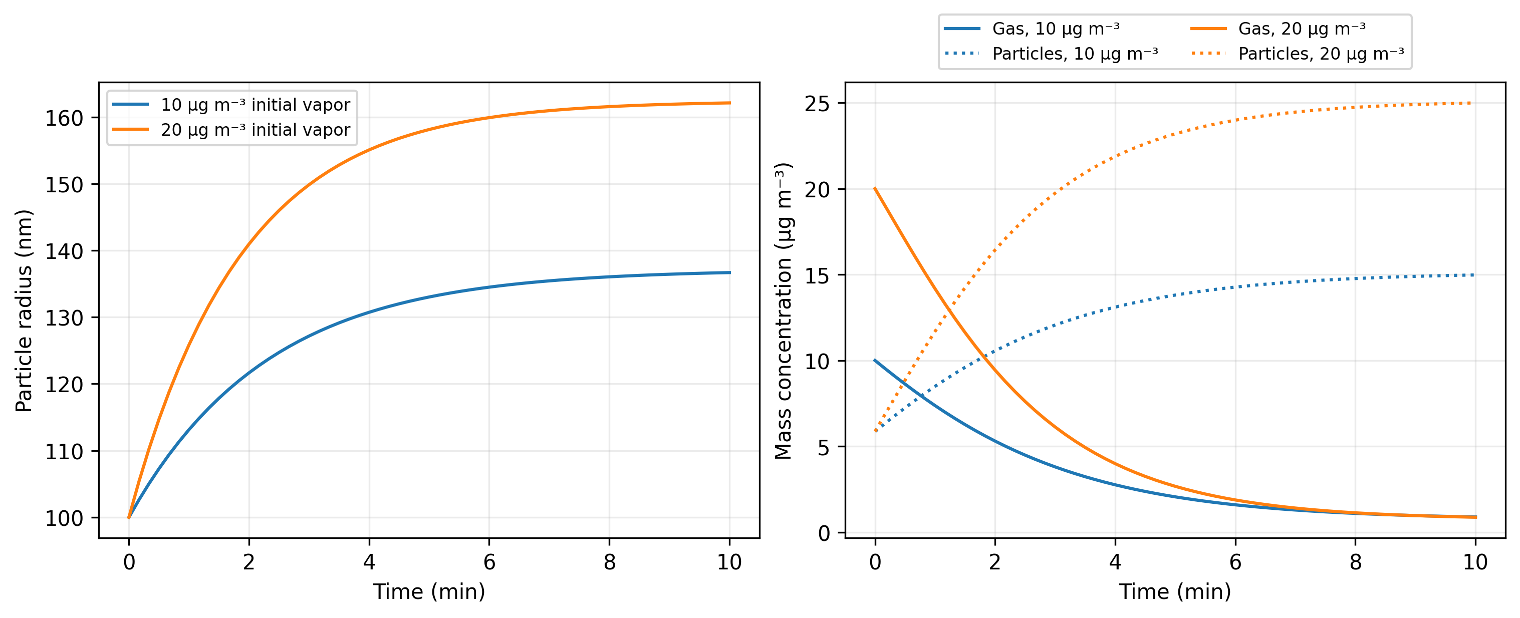
Run this downloaded script to retain two analysis files, two exact-restart
files and a PNG in first-cpu-results/. In a checkout, import simulate and
supply your own destination. To investigate volatility next, change the
saturation vapor pressure, rerun, and compare the remaining vapor as well as
radius. This run grows the particles from 100 nm to about 136.69 nm for
10 µg m⁻³ vapor and 162.13 nm for 20 µg m⁻³. Final vapor remains about
0.89 and 0.87 µg m⁻³, respectively. A physical prediction for a named compound
needs measured or otherwise
justified properties and an independent experimental comparison.
Prerequisites: native state and condensation physics.
Explore this topic: CPU workflows · Condensation and evaporation