

Follow droplets through one wet–dry chamber cycle
Follow droplets through one wet–dry chamber cycle
Section titled “Follow droplets through one wet–dry chamber cycle”What changes when hygroscopic seeds encounter a supersaturated vapor reservoir and then a drier one? This example couples condensation, evaporation, and rectangular-chamber wall removal, following individual particle sizes and the remaining gas-phase water. It provides a scaffold for reasoning about water exchange and survival in a chamber.
The two humidity settings initialize phases; they are not held fixed by a continuous controller. Each condensation step conserves its mapped species, whereas wall removal and the imposed humidity reset open that inventory. Adaptive ROS3 resolves condensation inside each 0.1 s wall-loss/output interval. Its local error control is distinct from convergence of the outer stochastic wall-loss schedule and from a quantitative activation threshold.
Start with condensation and rectangular wall loss if either process is unfamiliar. This example adds their interaction, not a validation against chamber measurements.
Make the sampling choices reproducible
Section titled “Make the sampling choices reproducible”Use NumPy for the sampled seed population and an explicit generator for wall removal. Fixed seeds make this particular realization repeatable under the same implementation. Estimating stochastic uncertainty would require an ensemble of independent realizations, which is not run here.
Python · section 1
import copy
import matplotlib.pyplot as pltimport numpy as npimport particula as parfrom particula.dynamics.condensation.species_mapping import (    CondensationSpeciesMap,)from particula.execution.splitting import condensation_flow
# Optional: uncomment if many steps and you want a progress bar# from tqdm import tqdm
# Plot style (Tailwind gray palette)TAILWIND = par.util.colors.TAILWINDbase_color = TAILWIND["gray"]["600"]plt.rcParams.update(    {        "text.color": base_color,        "axes.labelcolor": base_color,        "figure.figsize": (5, 4),        "font.size": 14,        "axes.edgecolor": base_color,        "xtick.color": base_color,        "ytick.color": base_color,        "pdf.fonttype": 42,        "ps.fonttype": 42,        "savefig.dpi": 150,    })
np.random.seed(100)  # reproducibility for sampling and wall-loss RNG
Define the geometry used by wall loss
Section titled “Define the geometry used by wall loss”The wall-loss model uses a 2 m × 1 m × 1 m chamber and an eddy-loss parameter of 0.001 s⁻¹. Particle removal is stochastic in the resolved representation. Keep this geometry distinct from the represented aerosol sample volume set below: one controls the loss coefficients, the other converts particle counts and gas concentration into an extensive inventory.
Python · section 2
# Geometry (meters)chamber_dims = (2.0, 1, 1)chamber_volume = np.prod(chamber_dims)print("Chamber volume (m^3):", chamber_volume)
# Rectangular wall-loss strategywall_loss_strategy = (    par.dynamics.RectangularWallLossBuilder()    .set_chamber_dimensions(chamber_dims)    .set_wall_eddy_diffusivity(0.001, "1/s")    .set_distribution_type("particle_resolved")    .build())wall_loss = par.dynamics.WallLoss(wall_loss_strategy=wall_loss_strategy)
Chamber volume (m^3): 2.0Put solute effects and water in aligned species lanes
Section titled “Put solute effects and water in aligned species lanes”Each particle contains ammonium sulfate, sucrose, and water, in that order. κ=[0.61, 0.10, 0] supplies an illustrative hygroscopicity model; densities are kg/m³ and molar masses kg/mol. Water is lane 2, and its own κ is unused. Solute activity and the later Kelvin surface correction both enter the condensation calculation. These fixed values do not describe every concentration or temperature dependence of the named materials.
Python · section 3
kappa = np.array([0.61, 0.10, 0.0])density = np.array([1770.0, 1587.0, 997.0]) # kg/m^3molar_mass = np.array([0.13214, 0.3423, 0.018015]) # kg/molactivity_params = ( par.particles.ActivityKappaParameterBuilder() .set_kappa(kappa) .set_density(density, "kg/m^3") .set_molar_mass(molar_mass, "kg/mol") .set_water_index(2) .build())Build a sampled dry population and its vapor reservoir
Section titled “Build a sampled dry population and its vapor reservoir”Sample 1000 dry radii from a lognormal distribution with 100 nm mode radius and geometric standard deviation 1.5. The dry material is 60% ammonium sulfate and 40% sucrose by volume, converted to species masses using their densities. Water starts at zero. The gas adds an unmapped air lane as well as the three mapped particle species.
The represented sample volume is 0.25 m³, distinct from the 2 m³ chamber geometry above. Constant water-like surface tension is assumed. The inventory helper combines weighted particle mass with gas concentration times sample volume, in kg; this is the quantity compared around each condensation step.
Python · section 4
# Sample particle radii from a lognormal distribution# This is more realistic than manually spaced diametersn_particles = 1000  # keep modest for speednp.random.seed(42)dry_radius = par.particles.get_lognormal_sample_distribution(    mode=np.array([100e-9]),  # 100 nm mode radius (typical CCN seed size)    geometric_standard_deviation=np.array(        [1.5]    ),  # typical GSD for accumulation mode    number_of_particles=np.array([1.0]),  # single mode    number_of_samples=n_particles,)
# Seed masses per particle (kg) from sampled radii# Species: ammonium sulfate, sucrose, water (matches kappa array order)volume_per_particle = 4 / 3 * np.pi * dry_radius**3# 60% ammonium sulfate, 40% sucrose by volume in dry seedammonium_sulfate_mass = 0.6 * volume_per_particle * density[0]  # kgsucrose_mass = 0.4 * volume_per_particle * density[1]  # kgwater_mass0 = np.zeros_like(dry_radius)  # start dryseed_mass = np.stack([ammonium_sulfate_mass, sucrose_mass, water_mass0], axis=1)
# Temperature and pressuretemperature = 298.15  # Ktotal_pressure = 101325.0  # Pa
# Create partitioning gas species (3 species to match particle species)# AS and sucrose have negligible vapor pressure but must be included for validationvapor_strategies = [    par.gas.ConstantVaporPressureStrategy(1e-30),    par.gas.ConstantVaporPressureStrategy(1e-30),    par.gas.WaterBuckVaporPressureBuilder().build(),    par.gas.ConstantVaporPressureStrategy(101325.0),]gas = par.gas.GasData(    name=["ammonium_sulfate", "sucrose", "water", "air"],    molar_mass=np.append(molar_mass, 0.029),    partitioning=np.array([True, True, True, False]),    concentration=np.array([[1e-30, 1e-30, 0.01, 1.2]]),)environment = par.gas.EnvironmentData(    temperature=np.array([temperature]),    pressure=np.array([total_pressure]),    saturation_ratio=np.zeros((1, 4)),)
# Create surface strategy for Kelvin effectsurface_strategy = (    par.particles.SurfaceStrategyVolumeBuilder()    .set_surface_tension(0.072, "N/m")  # water surface tension    .set_density(density, "kg/m^3")    .build())
# Build particle representation with lognormal-sampled particles# Represented sample volume differs from the geometry used for loss coefficients.chamber_volume = 0.25  # m³, retained represented volumeparticles = par.particles.create_resolved_particle_data(    masses=seed_mass,    density=density,    volume=chamber_volume,)aerosol = par.Aerosol(particles=particles, gas=gas, environment=environment)wall_loss_strategy.random_generator = np.random.default_rng(42)

def species_inventory(aero):    """Extensive inventory for the three mapped species, kg."""    return np.sum(        aero.particles.masses * aero.particles.concentration[..., None], axis=1    ) + (aero.gas.concentration[:, :3] * aero.particles.volume[:, None])

print(    "Particle slots:", n_particles, "represented volume (m^3):", chamber_volume)print("Gas species:", ", ".join(gas.name))
Particle slots: 1000 represented volume (m^3): 0.25
Gas species: ammonium_sulfate, sucrose, water, airSet phase boundaries without imposing a continuous RH ramp
Section titled “Set phase boundaries without imposing a continuous RH ramp”The configured strategy supplies continuous particle/gas mass rates to ROS3; its randomized staggered finite-step sweeps are not executed. Its explicit species map excludes air. Each phase spans exactly 30 s. Condensation uses adaptive accepted steps; wall removal and observation retain 0.1 s intervals. The vapor reset occurs at t=30 s after the wet interval has finished. Water vapor is initialized at 100.4% saturation and reset to 85% at the phase boundary. Between resets it evolves through mass transfer.
The conversion from vapor pressure to concentration uses the ideal-gas relation at 298.15 K. Thus the lower plot’s effective RH is a diagnostic of the changing gas reservoir, not an independently prescribed trajectory.
Python · section 5
# Full gas molar masses include air; the explicit map selects the three# particle species (ammonium sulfate, sucrose, water).condensation_strategy = par.dynamics.CondensationIsothermalStaggered(    molar_mass=gas.molar_mass.copy(),    diffusion_coefficient=2.4e-5,    accommodation_coefficient=1.0,    theta_mode="random",    num_batches=4,    random_state=42,    update_gases=True,    activity_strategy=activity_params,    surface_strategy=surface_strategy,    vapor_pressure_strategy=vapor_strategies,    species_map=CondensationSpeciesMap(        tuple(gas.name), ((0, 0), (1, 1), (2, 2))    ),)condensation = par.dynamics.MassCondensation(    condensation_strategy=condensation_strategy)growth_flow = condensation_flow(    "water_exchange",    condensation_strategy,    method="ros3",    rtol=1e-5,    particle_atol=1e-25,    gas_atol=1e-12,    first_step=1e-6,    max_step=0.1,)
# Time gridt_activation = 30.0  # st_deactivation = 30.0  # sdt = 0.1  # s (keeps total steps manageable)t = np.arange(0.0, t_activation + t_deactivation + dt, dt)n_steps = t.size
# Phase transition index (when we switch from activation to deactivation)activation_steps = int(t_activation / dt)
# RH targets (used to set initial gas concentrations at phase boundaries)rh_activation_target = 1.004  # 100.4% RH - supersaturatedrh_deactivation_target = 0.85  # 85% RH - subsaturated
# Calculate saturation vapor pressure and target water concentrationsp_sat_water = par.gas.get_buck_vapor_pressure(temperature)  # Pa# Convert to mass concentration: c = p * M / (R * T)R_gas = 8.314  # J/(mol*K)c_sat_water = p_sat_water * molar_mass[2] / (R_gas * temperature)  # kg/m^3
# Initial water concentration for activation phase (supersaturated)c_water_activation = rh_activation_target * c_sat_water# Water concentration for deactivation phase (subsaturated)c_water_deactivation = rh_deactivation_target * c_sat_water
print(f"Saturation vapor pressure: {p_sat_water:.1f} Pa")print(f"Saturation concentration: {c_sat_water * 1e3:.4f} g/m^3")print(    f"Activation concentration (RH={rh_activation_target}): {c_water_activation * 1e3:.4f} g/m^3")print(    f"Deactivation concentration (RH={rh_deactivation_target}): {c_water_deactivation * 1e3:.4f} g/m^3")
Saturation vapor pressure: 3168.5 Pa
Saturation concentration: 23.0275 g/m^3
Activation concentration (RH=1.004): 23.1196 g/m^3
Deactivation concentration (RH=0.85): 19.5734 g/m^3Track exchange and removal with different checks
Section titled “Track exchange and removal with different checks”At every step, compare the mapped particle-plus-gas inventory immediately before and after condensation at rtol=10⁻¹² and atol=10⁻³⁰ kg. Then apply wall loss and check that it cannot add particle mass. Air must remain unchanged. These local checks deliberately exclude the external water reset from a closed-system conservation claim.
Store particle masses, equivalent spherical diameters, and gas water for the same times. Zero-mass removed particles have zero plotted diameter. The saved realization reports its peak diameter and surviving slots below. These outcomes belong to this setup and random seed, not general chamber performance estimates. Particle tolerance is kg per particle; gas tolerance is kg/m³.
Python · section 6
n_particles = aerosol.particles.masses[0].copy().shape[0]diam_hist = np.empty((n_steps, n_particles))mass_hist = np.empty((n_steps, n_particles, seed_mass.shape[1]))gas_conc_hist = np.empty(n_steps)  # track gas-phase water concentration

def masses_to_diameter(masses: np.ndarray) -> np.ndarray:    """Convert speciated masses per particle to an equivalent spherical diameter.
    Particles with zero total mass are assigned a diameter of 0 to avoid    division-by-zero and NaN propagation when wall loss removes particles.    """    # total mass per particle    total_mass = masses.sum(axis=1)    # mask for particles that actually contain mass    nonzero = total_mass > 0
    # initialize diameters as zeros (for zero-mass particles this remains 0)    diameters = np.zeros_like(total_mass, dtype=float)
    if np.any(nonzero):        masses_nz = masses[nonzero]        total_mass_nz = total_mass[nonzero]        inv_bulk_density = (masses_nz / density).sum(axis=1) / total_mass_nz        bulk_density = 1.0 / inv_bulk_density        volume = total_mass_nz / bulk_density        diameters[nonzero] = (6 * volume / np.pi) ** (1 / 3)
    return diameters

def set_water_concentration(    aer: par.Aerosol, concentration: float) -> par.Aerosol:    """Set the gas-phase water vapor concentration in the atmosphere."""    aer.gas.concentration[0, 2] = concentration    return aer

# Initialize aerosol state with activation-phase water concentrationaerosol_state = copy.deepcopy(aerosol)aerosol_state = set_water_concentration(aerosol_state, c_water_activation)
# Record initial statemass_hist[0] = aerosol_state.particles.masses[0].copy()diam_hist[0] = masses_to_diameter(mass_hist[0])gas_conc_hist[0] = aerosol_state.gas.concentration[0, 2]
# Run simulation - condensation strategy tracks gas-phase mass internallyfor i in range(1, n_steps):    # Condensation handles mass transfer and updates gas concentration internally    before_condensation = species_inventory(aerosol_state)    aerosol_state = growth_flow.advance(aerosol_state, float(t[i - 1]), dt)    np.testing.assert_allclose(        species_inventory(aerosol_state),        before_condensation,        rtol=1e-12,        atol=1e-30,    )    before_wall = aerosol_state.particles.masses.copy()    aerosol_state = wall_loss.execute(aerosol_state, time_step=dt)    assert np.all(aerosol_state.particles.masses <= before_wall)    np.testing.assert_allclose(        aerosol_state.gas.concentration[0, 3], 1.2, rtol=0, atol=0    )
    # Finish the wet interval before applying the instantaneous reservoir reset.    # The row at the event shows its right-hand gas value and accepted particles.    if i == activation_steps:        aerosol_state = set_water_concentration(            aerosol_state, c_water_deactivation        )        print(f"Dry reservoir imposed at t={t[i]:.1f} s")
    mass_hist[i] = aerosol_state.particles.masses[0].copy()    diam_hist[i] = masses_to_diameter(mass_hist[i])    gas_conc_hist[i] = aerosol_state.gas.concentration[0, 2]
peak_idx = int(np.nanargmax(diam_hist.max(axis=1)))peak_diam = diam_hist[peak_idx].max()print(f"Peak diameter: {peak_diam * 1e6:.2f} um at t={t[peak_idx]:.1f} s")
survivors = np.isfinite(mass_hist[-1].sum(axis=1)) & (    mass_hist[-1].sum(axis=1) > 0)print("Survivors:", survivors.sum(), "of", n_particles)
Dry reservoir imposed at t=30.0 sPeak diameter: 23.19 um at t=30.0 s
Survivors: 788 of 1000Read size histories beside the vapor history
Section titled “Read size histories beside the vapor history”The upper panel shows sampled particle diameters and the lower panel shows effective RH. Shading marks the wet and dry phases. Growth consumes gas water; the imposed reset changes the reservoir, after which evaporation can return water to the gas. Removal is a separate sink.
Condensation now uses the stiff adaptive method rather than one fixed condensation update per plotted interval. Check tolerance refinement before interpreting small size reversals, and refine the outer wall-loss schedule separately before inferring a converged activation criterion.
Python · section 7
colors = [    TAILWIND["blue"]["500"],    TAILWIND["amber"]["500"],    TAILWIND["emerald"]["500"],    TAILWIND["rose"]["500"],    TAILWIND["violet"]["500"],]
fig, (ax1, ax2) = plt.subplots(2, 1, figsize=(6, 8), sharex=True)
# Plot particle diametersfor j in range(n_particles):    color = colors[j % len(colors)]    ax1.plot(t / 60, diam_hist[:, j] * 1e6, color=color, alpha=0.6, linewidth=1)ax1.axvspan(    0,    t_activation / 60,    color=TAILWIND["gray"]["200"],    alpha=0.3,    label="activation",)ax1.axvspan(    t_activation / 60,    (t_activation + t_deactivation) / 60,    color=TAILWIND["gray"]["300"],    alpha=0.2,    label="deactivation",)ax1.set_ylabel("Particle diameter (um)")ax1.set_title("Activation -> Deactivation")ax1.legend()
# Plot gas-phase water concentration (as effective RH)effective_rh = gas_conc_hist / c_sat_waterax2.plot(t / 60, effective_rh * 100, color=TAILWIND["blue"]["600"], linewidth=2)ax2.axhline(    100, color=TAILWIND["gray"]["400"], linestyle="--", label="saturation")ax2.axvspan(0, t_activation / 60, color=TAILWIND["gray"]["200"], alpha=0.3)ax2.axvspan(    t_activation / 60,    (t_activation + t_deactivation) / 60,    color=TAILWIND["gray"]["300"],    alpha=0.2,)ax2.set_xlabel("Time (minutes)")ax2.set_ylabel("Effective RH (%)")ax2.set_title("Gas-phase water (equilibrates internally)")ax2.legend()
plt.tight_layout()plt.show()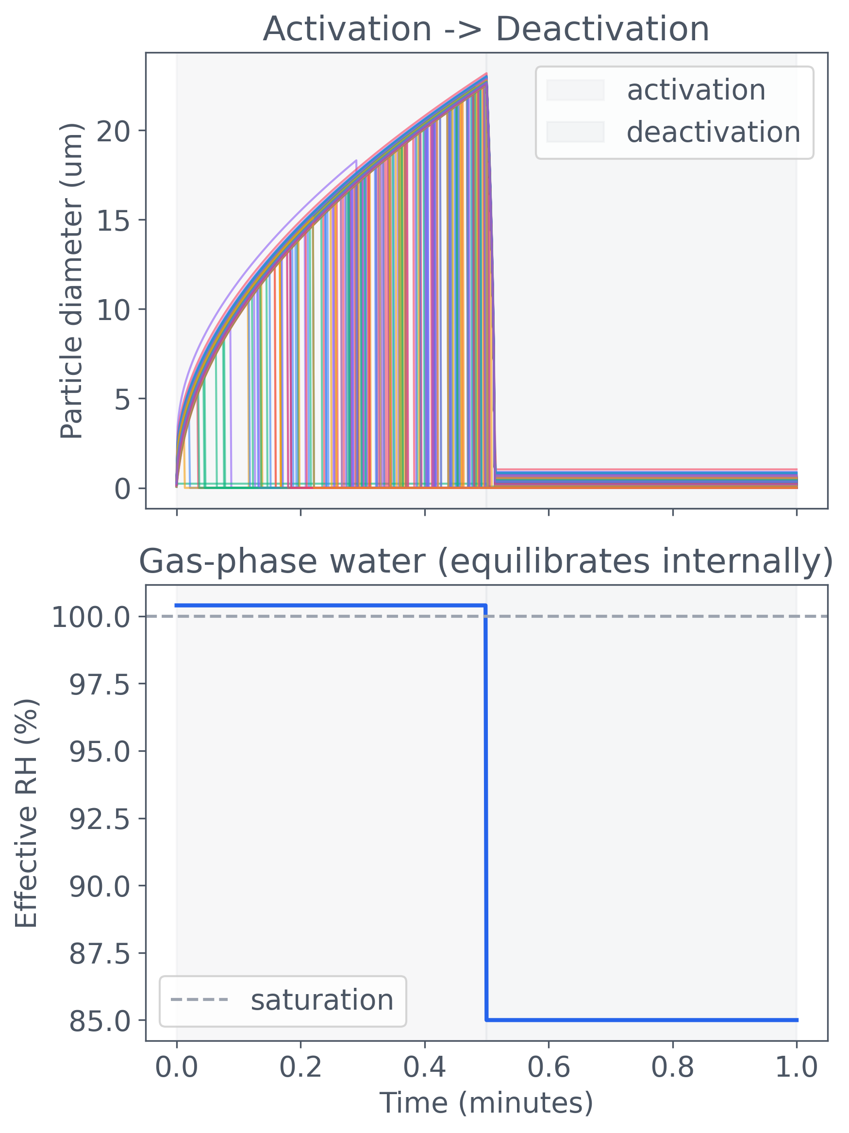
Separate an inventory check from a wet-to-dry mass ratio
Section titled “Separate an inventory check from a wet-to-dry mass ratio”The final block checks finite masses and a bounded survivor count, and reports peak diameter. It does not assert a 5 µm activation threshold or convergence. The printed “mass remaining” divides final wet particle mass by initial dry seed mass, so it can greatly exceed 100%. It is neither a wall-deposition fraction nor a measure of mass-conservation error. Conservation of the mapped species was checked separately around each condensation operation.
Python · section 8
# Peak diameter check - particles should grow during activationprint(f"Peak diameter: {np.nanmax(diam_hist) * 1e6:.2f} um")
# Survival sanity - wall loss may remove particlessurvivor_mask = (mass_hist[-1].sum(axis=1) > 0) & np.isfinite(    mass_hist[-1].sum(axis=1))n_survivors = survivor_mask.sum()print(f"Survivors after wall loss: {n_survivors} of {n_particles}")if not (0 <= n_survivors <= n_particles):    raise ValueError(f"Invalid survivor count: {n_survivors}")
# Finite values checkif not np.isfinite(mass_hist).all():    raise ValueError("Non-finite masses found")
# Particle mass ratio includes water exchange and prescribed humidity resets;# it is not a measure of wall deposition. Closed condensation is checked above.initial_total_mass = seed_mass.sum()final_total_mass = mass_hist[-1].sum()mass_remaining = final_total_mass / initial_total_mass * 100print(f"Mass remaining: {mass_remaining:.1f}% (includes water uptake and loss)")
# Note: With wall loss enabled, mass is NOT conserved by design# Wall loss is a stochastic process that removes particles from the systemprint("Simulation completed successfully.")
Peak diameter: 23.19 um
Survivors after wall loss: 788 of 1000
Mass remaining: 180.6% (includes water uptake and loss)
Simulation completed successfully.What this cycle supports—and what to investigate next
Section titled “What this cycle supports—and what to investigate next”The calculation connects a humidity change to particle water exchange while wall removal reduces the surviving population. The adaptive result resolves smooth dry-phase relaxation. The independent wet–dry accuracy comparison shows why mass conservation alone cannot establish temporal accuracy, and compares ROS2 and ROS3 work at the same tolerances.
Before using this setup to interpret an experiment, reduce the timestep and compare peak diameter, dry-phase size histories, and gas water. Then repeat across random seeds to quantify survival uncertainty. Keep humidity additions and removals in an explicit external-water budget. The multiple-cycle example extends the forcing and composition comparisons, but still needs those numerical and experimental checks for a quantitative chamber study.
Explore this topic: Chamber experiments · Condensation and evaporation · Wall loss and dilution