

How does water uptake change organic aerosol partitioning?
How does water uptake change organic aerosol partitioning?
Section titled “How does water uptake change organic aerosol partitioning?”At fixed total organic loading, changing water activity can change both aerosol
water and the amount of organic material in the condensed phase. Here a
five-component volatility distribution is solved at equilibrium, first at
Use the BAT phase-property walkthrough to understand the activity coefficients and phase weights. This functional calculation does not require an aerosol container and does not predict a condensation timescale. It uses the reduced thermodynamic framework of Gorkowski, Preston, and Zuend (2019).
Python · section 1
# In Colab uncomment the following command to install particula:# Install from the repository root: `python -m pip install -e ".[extra]"`# Importing necessary librariesimport matplotlib.pyplot as plt  # For creating plots and visualizationsimport numpy as np  # For numerical operations
# For partitioning calculations in liquid-vapor equilibriumfrom particula.equilibria import partitioningfrom particula.particles.properties.organic_density_module import (    get_organic_density_array,)  # For calculating species density
Span volatility while fixing the available organic mass
Section titled “Span volatility while fixing the available organic mass”The dry saturation concentrations
O:C and estimated density supply the activity calculation. The density helper returns kg/m³ using its default elemental assumptions. The generic components are illustrative, not a measured speciation or fitted emission mixture.
Python · section 2
# Defining system parametersc_star_j_dry = np.array(    [1e-6, 1e-4, 1e-1, 1e2, 1e4], dtype=float)  # Volatility distribution in ug/m3# Total concentration in ug/m3concentration_organic_matter = np.array([1, 5, 10, 15, 10], dtype=float)oxygen2carbon = np.array([0.2, 0.3, 0.5, 0.4, 0.4])  # Oxygen to carbon ratios
molar_mass = np.array([200, 200, 200, 200, 200])  # Molar mass in g/molwater_activity_desired = np.array([0.8])  # Desired water activitymolar_mass_ratio = 18.015 / np.array(molar_mass)  # Molar mass ratio
# Calculate the density of organic compoundsdensity = get_organic_density_array(    molar_mass,    oxygen2carbon,    hydrogen2carbon=None,    nitrogen2carbon=None,)
Connect phase properties to mass partitioning
Section titled “Connect phase properties to mass partitioning”At
The saved calculation gives about 24.22 µg/m³ condensed organic material and 9.41 µg/m³ aerosol water. Organic mass is bounded by the 41 µg/m³ total; water comes from the imposed equilibrium activity rather than that organic inventory. These values depend on the chosen surrogate mixture.
Python · section 3
# Calculate the properties needed for liquid-vapor partitioninggamma_organic_ab, mass_fraction_water_ab, q_ab = (    partitioning.get_properties_for_liquid_vapor_partitioning(        water_activity_desired=water_activity_desired,        molar_mass=molar_mass,        oxygen2carbon=oxygen2carbon,        density=density,    ))
# The optimization the partition coefficients, i.e. the partitioning calculationalpha_opt, beta_opt, system_opt, fit_result = (    partitioning.liquid_vapor_partitioning(        c_star_j_dry=c_star_j_dry,        concentration_organic_matter=concentration_organic_matter,        molar_mass=molar_mass,        gamma_organic_ab=gamma_organic_ab,        mass_fraction_water_ab=mass_fraction_water_ab,        q_ab=q_ab,        partition_coefficient_guess=None,    ))
print(f"mass in organic aerosol [ug/m3]: {system_opt[0]}")print(f"mass in water [ug/m3]: {system_opt[1]}")
mass in organic aerosol [ug/m3]: 24.216782218329037
mass in water [ug/m3]: 9.407806893154259Repeat equilibria across water activity
Section titled “Repeat equilibria across water activity”Each of the 50 points from
The arrays retain condensed mass concentrations, not activity coefficients. Changing humidity influences those masses through both phase properties and partitioning. No parameter fitting to observations occurs in this sweep.
Python · section 4
# Calculating activity coefficients across a range of RH values# Range of water activity (RH/100)water_activity_curve = np.linspace(0.01, 0.99, 50)total_oa_concentration = np.empty([len(water_activity_curve), 1], dtype=float)water_concentration = np.empty([len(water_activity_curve), 1], dtype=float)
for i, water_activity in enumerate(water_activity_curve):    # Get properties for liquid-vapor partitioning at each RH value    gamma_organic_ab, mass_fraction_water_ab, q_ab = (        partitioning.get_properties_for_liquid_vapor_partitioning(            water_activity_desired=water_activity,            molar_mass=molar_mass,            oxygen2carbon=oxygen2carbon,            density=density,        )    )
    # Optimize the partition coefficients for each RH value    alpha_opt, beta_opt, system_opt, fit_result = (        partitioning.liquid_vapor_partitioning(            c_star_j_dry=c_star_j_dry,            concentration_organic_matter=concentration_organic_matter,            molar_mass=molar_mass,            gamma_organic_ab=gamma_organic_ab,            mass_fraction_water_ab=mass_fraction_water_ab,            q_ab=q_ab,            partition_coefficient_guess=None,        )    )
    # Record the total organic and water concentration    total_oa_concentration[i] = system_opt[0]    water_concentration[i] = system_opt[1]
print("Calculation complete")
Calculation completeInterpret the two concentration scales
Section titled “Interpret the two concentration scales”The green curve uses the left axis for organic aerosol and the blue curve uses the right axis for aerosol water, both in µg/m³. Follow each axis separately: a line crossing is not equality of concentrations. The high-activity water response illustrates how strongly water uptake can change while organic mass remains constrained by a fixed inventory.
The plotted states are equilibrium predictions for these inputs, not evidence of how quickly an ambient aerosol responds or of validated multiphase kinetics.
Python · section 5
fig, ax = plt.subplots()ax.plot(    water_activity_curve,    total_oa_concentration,    label="total organic concentration",    color="green",)aw = ax.twinx()aw.plot(    water_activity_curve,    water_concentration,    label="water concentration",    color="blue",)plt.legend(loc="upper left")ax.set_xlabel("Water activity")
handles, labels = ax.get_legend_handles_labels()aw_handles, aw_labels = aw.get_legend_handles_labels()handles.extend(aw_handles)labels.extend(aw_labels)plt.legend(handles, labels, loc="upper left")
ax.set_ylabel("organic aerosol concentration [ug/m3]")aw.set_ylabel("aerosol water concentration [ug/m3]")plt.show()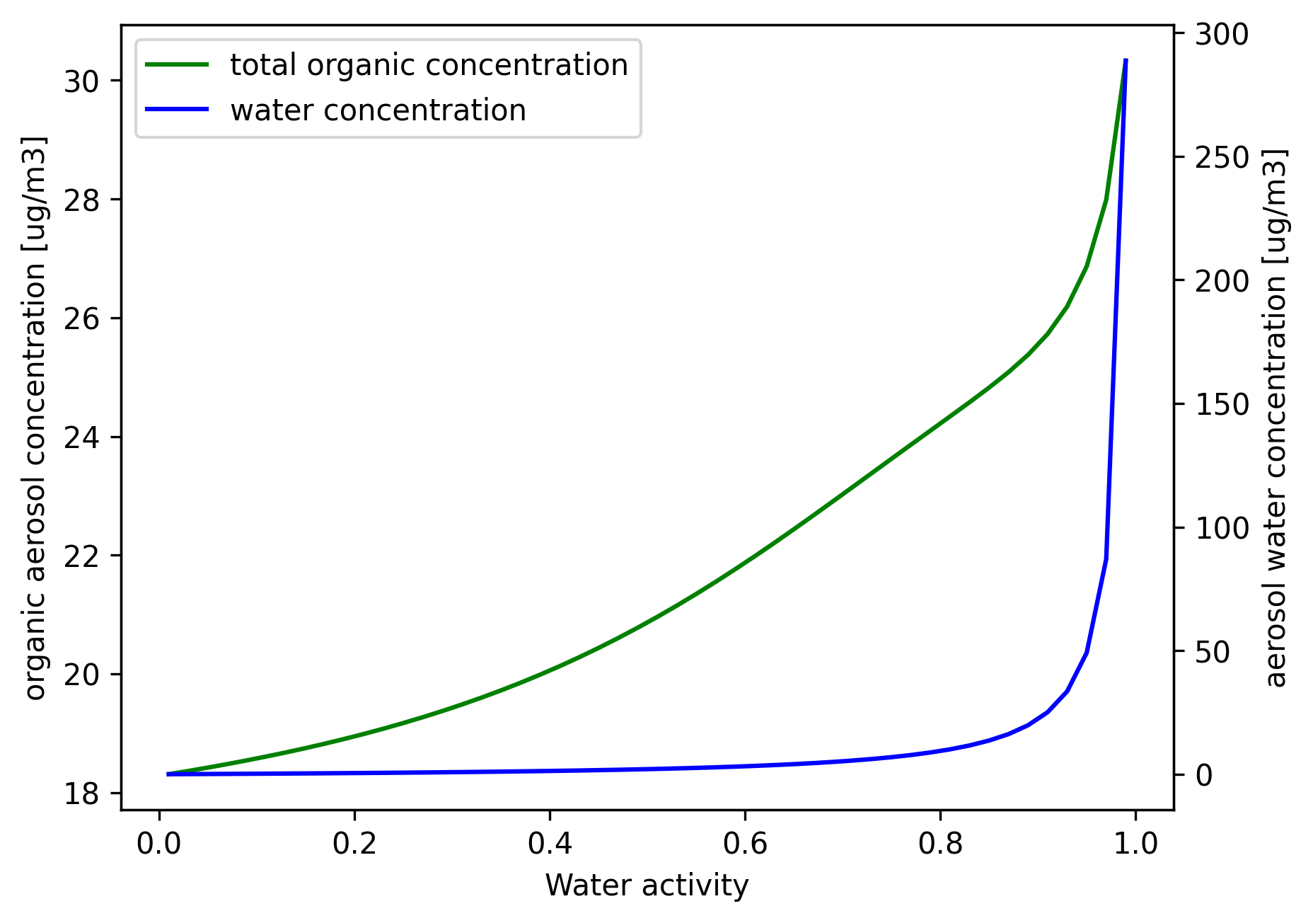
Use the equilibrium curve as a bounded reference
Section titled “Use the equilibrium curve as a bounded reference”Water activity affects more than aerosol water: it also changes the equilibrium organic partitioning problem. The final checks require finite, nonnegative masses and organic concentration no greater than the available inventory. Those bounds are necessary checks, not proof of solver convergence at every point or agreement with measured aerosol composition.
For a research extension, vary the total organic loading while preserving its species ratios, then compare the fraction condensed at each water activity. Record solver success and residuals as well as mass bounds; compare the result with a measured humidity-dependent partitioning curve. A time-dependent condensation example would address the separate question of approaching those equilibria.
Python · section 6
# Check finite, physically bounded condensed organic mass across the RH sweep.assert np.all(np.isfinite(total_oa_concentration))assert np.all(total_oa_concentration >= 0)assert np.all(total_oa_concentration <= concentration_organic_matter.sum())assert np.all(np.isfinite(water_concentration))assert np.all(water_concentration >= 0)Explore this topic: Phase equilibrium and partitioning