

Cooling, heating and vapor pulses across sixteen boxes
Download Python script · Download script with helper and data files (.zip)
Cooling, heating and vapor pulses across sixteen boxes
Section titled “Cooling, heating and vapor pulses across sixteen boxes”When vapor and temperature change externally, how can you distinguish a particle response from mass supplied by the forcing? This example builds an open-system inventory and compares response histories across boxes. Start with the prepared interface; the key scientific step is recording each imposed gas replacement before interpreting condensation.
This study uses 49,152 active resolved particles, four particle materials and five gas lanes. Only water exchanges between gas and particle material; the other materials and spectator gases provide independent accounting checks. The complete trajectory contains 6,000 steps of 1 microsecond (0.006 s total). This is an illustrative rapid forcing experiment.
A prescribed temperature cycle cools the boxes toward 275 K, heats them toward 310 K, then returns toward 298 K. Each box has a fixed temperature offset, updated at 120 fixed control times. Water gas is replaced twice, at nominal saturation ratios 1.6 and 0.8. These are external mass sources or sinks, so their actual per-box mass changes enter the ledger before dilution.
update_environment and update_gas are explicit upload boundaries.
Exact dilution keeps its fixed schedule and can replay a captured event graph.
Condensation uses adaptive ROS3, with explicit state transfers every cycle;
its rejected trials never repeat dilution. This host-controlled composition
demonstrates correctness and error control, not fully resident acceleration.
The study helpers and plotting code are included in the downloadable ZIP.
A second run halves the outer timestep and tightens the condensation relative
tolerance from 1e-5 to 1e-7, retaining the exact control times. Every particle’s
final total mass must change by less than
1%, and every box’s final water vapor by less than 0.1%.
Python · section 1
"""Manually refreshed CUDA forcing and independent-species-width study."""
import matplotlib.pyplot as pltimport warp as wpfrom scripts.docs_gpu_figures import history_figuresfrom scripts.gpu_studies.adaptive_trajectories import run_adaptive_forcingfrom scripts.gpu_studies.cases import StudyCase, build_case

def run_example():    """Run prescribed forcing and require every observed source/sink balance."""    case = StudyCase(        "time-varying-16",        "condensation",        16,        4096,        materials=4,        gases=5,        occupancy=0.75,        time_step=1e-6,        steps=6000,        heterogeneous=True,        experiment="forcing",    )    initial, _, processes = build_case(case)    report = run_adaptive_forcing(case, initial, processes)    history_figures(        report,        "Cooling and vapor pulses · " + wp.get_device("cuda:0").name,        forcing=True,    )    print(        "Shapes: particle materials",        initial.particles.masses.shape,        "gas species",        initial.gas.concentration.shape,    )    print("Timestep refinement:", report["refinement"])    plt.show()    return report
Interpret forcing separately from response
Section titled “Interpret forcing separately from response”Temperature is prescribed. Saturation is derived from the current gas and the water vapor-pressure law. A gas pulse is not spontaneous particle mass creation: the displayed inventory residual includes that external exchange. Final size distributions can retain different histories even after the temperatures approach each other. This illustrates finite-rate response; a predictive study should choose its timestep and forcing resolution for the physical timescales being investigated.
This manual CUDA refresh is excluded from routine CI execution.
Python · section 2
if __name__ == "__main__": run_example()Explicit cuda invocation
result = run_example()Maximum per-box, per-material inventory relative error: 1.1546319456101628e-14
Net prescribed water addition across boxes (kg): 1.1841560613752289e-11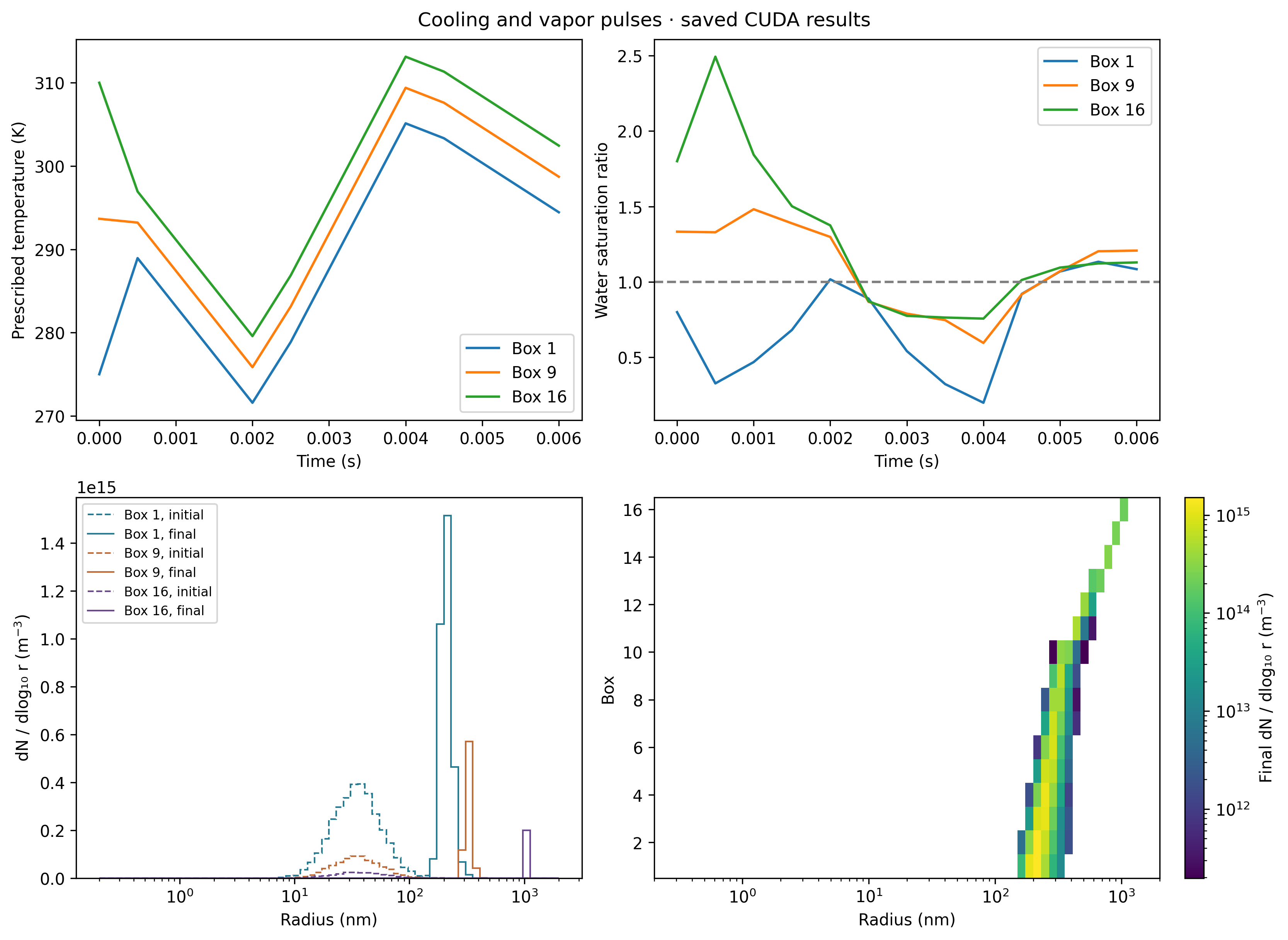
Use the forcing ledger to ask a different question
Section titled “Use the forcing ledger to ask a different question”The curves describe finite-rate response to a prescribed millisecond experiment; the inventory residual checks the accounting after external exchange and dilution. The refinement check bounds the two reported final-state changes for one timestep halving. It does not establish a timestep-independent response at every forcing boundary or validate this forcing as a chamber experiment. The saved full comparison gives maximum relative changes of 2.32×10⁻⁷ in final particle total mass and 8.86×10⁻⁹ in final water vapor. The respective coarse/fine inventory residuals are 1.15×10⁻¹⁴ and 2.93×10⁻¹⁴.
The figure retains 13 observations. Its zero-time point is the supplied initial state, before the first control update. Later points show completed cycles before the next scheduled update. Lines join those observations; they do not resolve all 120 control changes or the immediate response to each vapor pulse.
For a measured humidity pulse, supply its temperature and vapor histories, retain identical physical control times in a refinement run, and compare uptake lag and peak saturation as well as final mass. Compare with a temperature-only control to separate cooling from added water. The heterogeneous-box example shows the corresponding calculation without imposed vapor pulses.
Explore this topic: Prepared simulations