

Choose an activity model by the comparison it enables
Python · section 1
# Example workflow validation - edit-lint-sync-execute cycle verifiedChoose an activity model by the comparison it enables
Section titled “Choose an activity model by the comparison it enables”How does a composition assumption change the equilibrium pressure above an aerosol solution? This sequence compares ideal mole-fraction activity, a BAT organic–water approximation, and κ water activity, then connects activity to phase partitioning. The outcome is a way to design matched comparisons, not a universal ranking of models.
Activity is dimensionless and relates a component to a specified reference state. Evaporation or uptake depends on ambient vapor relative to the resulting surface equilibrium pressure; activity alone does not determine the direction of transfer. Read vapor pressure for that distinction. The configuration example focuses separately on strategies, builders, and factories.
Python · section 2
# Install particula if needed (uncomment for Colab)# Install from the repository root: `python -m pip install -e ".[extra]"`
import matplotlib.pyplot as pltimport numpy as npimport particula as par
# Set plot styleplt.style.use("seaborn-v0_8-whitegrid")
Establish an ideal mole-fraction reference
Section titled “Establish an ideal mole-fraction reference”For ideal mixing in the mole-fraction convention, aᵢ = xᵢ and the flat-interface equilibrium pressure is pᵢ = aᵢ pᵢ°. The initial binary example uses water (18.015 g mol⁻¹) and an illustrative 200 g mol⁻¹ organic. This is a chosen approximation, not evidence that the actual mixture is ideal.
Python · section 3
# Define species: water and organicmolar_mass = np.array([18.015e-3, 200.0e-3])  # kg/mol
# Create ideal molar activity strategyideal_strategy = par.particles.ActivityIdealMolar(    molar_mass=molar_mass,)
print(f"Strategy: {type(ideal_strategy).__name__}")print(f"Molar masses: {ideal_strategy.molar_mass * 1e3} g/mol")
Strategy: ActivityIdealMolar
Molar masses: [ 18.015 200. ] g/molConvert the composition before interpreting activity
Section titled “Convert the composition before interpreting activity”Both components contribute 0.5 µg m⁻³, but water has many more moles. The direct mole-fraction calculation provides an algebraic reference for the strategy; the water activity is about 0.9174, not 0.5.
Python · section 4
# Define mass concentrations (50% water, 50% organic by mass)mass = np.array([0.5e-9, 0.5e-9])  # kg/m^3
# Compute activityactivity = ideal_strategy.activity(mass_concentration=mass)
print(f"Mass concentrations: {mass * 1e9} ug/m^3")print(f"Activity values: water={activity[0]:.4f}, organic={activity[1]:.4f}")
# Verify activity equals mole fractionmoles = mass / molar_massmole_fractions = moles / np.sum(moles)print(    f"Mole fractions: water={mole_fractions[0]:.4f}, organic={mole_fractions[1]:.4f}")
Mass concentrations: [0.5 0.5] ug/m^3
Activity values: water=0.9174, organic=0.0826
Mole fractions: water=0.9174, organic=0.0826Read the composition sweep in its plotted coordinate
Section titled “Read the composition sweep in its plotted coordinate”The horizontal axis is water mass fraction, whereas ideal activity is mole fraction. Curvature in these plotted lines therefore does not demonstrate nonideality: it follows from the different molar masses. The two activities sum to one in this ideal binary model.
Python · section 5
# Calculate activity across composition rangewater_fractions = np.linspace(0.01, 0.99, 50)water_activities = []organic_activities = []
for wf in water_fractions:    mass = np.array([wf, 1.0 - wf]) * 1e-9    activity = ideal_strategy.activity(mass_concentration=mass)    water_activities.append(activity[0])    organic_activities.append(activity[1])
# Plotfig, ax = plt.subplots(figsize=(8, 5))ax.plot(water_fractions, water_activities, "b-", linewidth=2, label="Water")ax.plot(water_fractions, organic_activities, "r-", linewidth=2, label="Organic")ax.set_xlabel("Water Mass Fraction", fontsize=12)ax.set_ylabel("Activity", fontsize=12)ax.set_title("Ideal Activity (Raoult's Law)", fontsize=14)ax.legend(fontsize=11)ax.set_xlim(0, 1)ax.set_ylim(0, 1)plt.tight_layout()plt.show()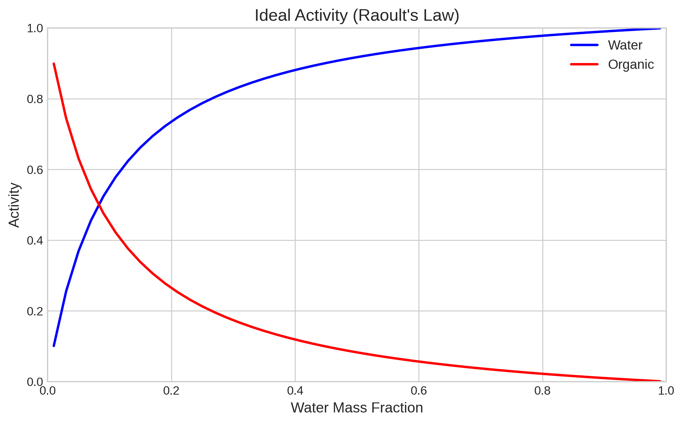
Introduce a composition-dependent activity coefficient
Section titled “Introduce a composition-dependent activity coefficient”BAT represents organic–water nonideality using reduced molecular descriptors; aᵢ = γᵢ xᵢ separates activity from its coefficient. This case uses organic molar mass 200 g mol⁻¹, O:C = 0.4, and density 1200 kg m⁻³ with the default functional-group assumption. The BAT model paper provides its scientific basis and scope.
ActivityNonIdealBinary returns organic activity only. Compare that scalar
with the organic entry from the ideal model, not with water activity.
Python · section 6
# Create non-ideal activity strategy using builderbat_strategy = (    par.particles.ActivityNonIdealBinaryBuilder()    .set_molar_mass(200.0, "g/mol")  # automatic unit conversion    .set_oxygen2carbon(0.4)  # O:C ratio    .set_density(1200.0, "kg/m^3")    .build())
print(f"Strategy: {type(bat_strategy).__name__}")print(f"Organic O:C ratio: {bat_strategy.oxygen2carbon}")
Strategy: ActivityNonIdealBinary
Organic O:C ratio: 0.4Compare one component at one composition
Section titled “Compare one component at one composition”At 50% water by mass, γ for the organic is computed by dividing BAT activity by the organic mole fraction. A departure from one measures the difference from the ideal reference at this composition. Neither value is a growth rate or a phase-separation criterion by itself.
Python · section 7
# Compute activities at 50% watermass = np.array([0.5, 0.5]) * 1e-9  # kg/m^3
ideal_activity = ideal_strategy.activity(mass_concentration=mass)# Note: BAT model returns only organic activity (scalar)bat_organic_activity = bat_strategy.activity(mass_concentration=mass)
print("At 50% water by mass:")print(    f"  Ideal activity:     water={ideal_activity[0]:.4f}, organic={ideal_activity[1]:.4f}")print(f"  Non-ideal (BAT):    organic={bat_organic_activity:.4f}")
# Compute activity coefficient for organicmoles = mass / np.array([18.015e-3, 200.0e-3])mole_frac = moles / np.sum(moles)gamma_organic = bat_organic_activity / mole_frac[1]print(f"\n  Organic activity coefficient: gamma={gamma_organic:.4f}")
At 50% water by mass:
Ideal activity: water=0.9174, organic=0.0826
Non-ideal (BAT): organic=0.1340
Organic activity coefficient: gamma=1.6214Compare organic activity across composition
Section titled “Compare organic activity across composition”Both curves below now represent organic activity for the same prescribed mass fractions. Their separation isolates the activity-model difference within the stated descriptor assumptions. Both curves describe the organic component, so the difference reflects the activity model at a matched composition.
Python · section 8
# Calculate activities across composition rangewater_fractions = np.linspace(0.1, 0.9, 40)
ideal_organic_comparison = []bat_organic = []
for wf in water_fractions:    mass = np.array([wf, 1.0 - wf]) * 1e-9    ideal_organic_comparison.append(        ideal_strategy.activity(mass_concentration=mass)[1]    )    # BAT returns organic activity (scalar), not water activity    bat_organic.append(float(bat_strategy.activity(mass_concentration=mass)))
# Plotfig, ax = plt.subplots(figsize=(8, 5))ax.plot(    water_fractions,    ideal_organic_comparison,    "b--",    linewidth=2,    label="Ideal Organic Activity",)ax.plot(    water_fractions,    bat_organic,    "r-",    linewidth=2,    label="Non-Ideal Organic Activity (BAT, O:C=0.4)",)ax.set_xlabel("Water Mass Fraction", fontsize=12)ax.set_ylabel("Activity", fontsize=12)ax.set_title("Activity: Ideal vs Non-Ideal (BAT)", fontsize=14)ax.legend(fontsize=11)ax.set_xlim(0, 1)ax.set_ylim(0, 1)plt.tight_layout()plt.show()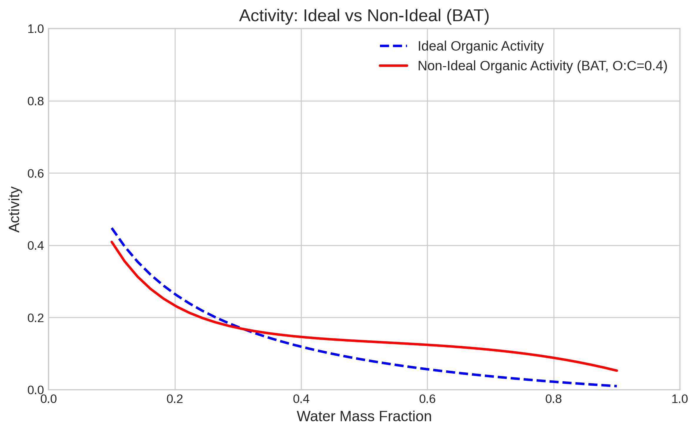
Test O:C sensitivity without changing molecular mass
Section titled “Test O:C sensitivity without changing molecular mass”The next panel varies O:C from 0.1 to 0.7 while keeping the other supplied descriptors fixed. All lines represent organic activity. Compare deviations from the ideal reference as a function of composition, rather than assuming one O:C value must be closer to ideal everywhere. Nonideal activity can exceed one in the chosen reference convention.
Python · section 9
# Test different O:C ratioso2c_values = [0.1, 0.3, 0.5, 0.7]water_fractions = np.linspace(0.1, 0.9, 40)
fig, ax = plt.subplots(figsize=(8, 5))
# Ideal reference (organic activity)ideal_organic = [    ideal_strategy.activity(mass_concentration=np.array([wf, 1 - wf]) * 1e-9)[1]    for wf in water_fractions]ax.plot(water_fractions, ideal_organic, "k--", linewidth=1.5, label="Ideal")
# BAT at different O:C ratios (returns organic activity)colors = plt.colormaps["viridis"](np.linspace(0.2, 0.8, len(o2c_values)))for o2c, color in zip(o2c_values, colors):    strat = (        par.particles.ActivityNonIdealBinaryBuilder()        .set_molar_mass(200.0, "g/mol")        .set_oxygen2carbon(o2c)        .set_density(1200.0, "kg/m^3")        .build()    )    bat_organic = [        float(strat.activity(mass_concentration=np.array([wf, 1 - wf]) * 1e-9))        for wf in water_fractions    ]    ax.plot(        water_fractions,        bat_organic,        "-",        color=color,        linewidth=2,        label=f"O:C={o2c}",    )
ax.set_xlabel("Water Mass Fraction", fontsize=12)ax.set_ylabel("Organic Activity", fontsize=12)ax.set_title("Effect of O:C Ratio on Organic Activity (BAT Model)", fontsize=14)ax.legend(fontsize=10, loc="lower right")ax.set_xlim(0, 1)ax.set_ylim(bottom=0)  # Non-ideal activity may exceed one.plt.tight_layout()plt.show()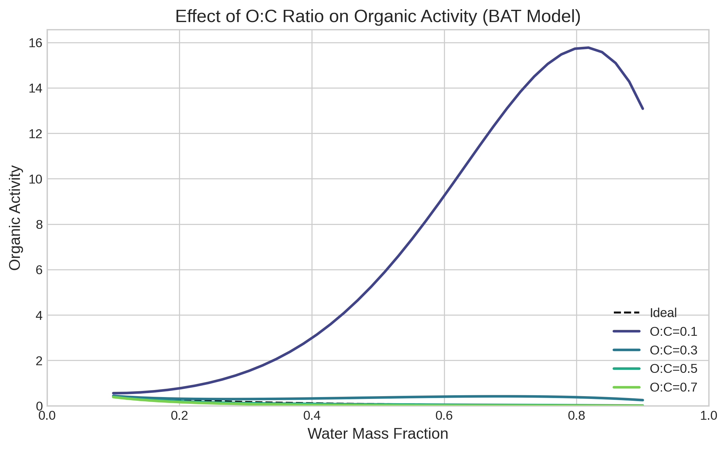
Use κ for a different question: water content and hygroscopicity
Section titled “Use κ for a different question: water content and hygroscopicity”The κ approximation describes water activity through a_w = V_w/(V_w + κV_s). It does not by itself provide a full electrolyte model or a curvature correction. The next case uses water and ammonium-sulfate properties, with κ = 0.61. That choice is a CCN-derived value summarized by Petters and Kreidenweis (2007), not a universal value at all compositions and phases.
Python · section 10
# Water + ammonium sulfate systemkappa_strategy = par.particles.ActivityKappaParameter(    kappa=np.array([0.0, 0.61]),  # water, (NH4)2SO4    density=np.array([1000.0, 1770.0]),  # kg/m^3    molar_mass=np.array([18.015e-3, 132.14e-3]),  # kg/mol    water_index=0,)
print(f"Strategy: {type(kappa_strategy).__name__}")print(f"Kappa values: {kappa_strategy.kappa}")
Strategy: ActivityKappaParameter
Kappa values: [0. 0.61]Change water content at fixed solute properties
Section titled “Change water content at fixed solute properties”Mass fractions are converted to volume fractions using the specified densities. The printed water activities increase as the salt is diluted. These are prescribed compositions, not a simulated humidity-driven growth trajectory.
Python · section 11
# Compute water activity at different water contentsprint("Water Activity for Water + Ammonium Sulfate:")print("Water Fraction | Water Activity")print("-" * 35)
for water_frac in [0.3, 0.5, 0.7, 0.9]:    mass = np.array([water_frac, 1.0 - water_frac]) * 1e-9    activity = kappa_strategy.activity(mass_concentration=mass)    print(f"    {water_frac:.1f}        |     {activity[0]:.4f}")
Water Activity for Water + Ammonium Sulfate:
Water Fraction | Water Activity
-----------------------------------
0.3 | 0.5543
0.5 | 0.7437
0.7 | 0.8713
0.9 | 0.9631Isolate κ in a generic solute sweep
Section titled “Isolate κ in a generic solute sweep”This plot changes κ at fixed solute density 1500 kg m⁻³ and molar mass 100 g mol⁻¹; it is a different system from the salt case above. Larger κ lowers water activity at fixed water mass fraction. The consequence for equilibrium uptake requires specifying ambient humidity and, for small particles, curvature.
Python · section 12
# Compare different kappa valueskappa_values = [0.1, 0.3, 0.61, 1.0]water_fractions = np.linspace(0.2, 0.95, 40)
fig, ax = plt.subplots(figsize=(8, 5))
colors = plt.colormaps["plasma"](np.linspace(0.2, 0.8, len(kappa_values)))for kappa, color in zip(kappa_values, colors):    strat = par.particles.ActivityKappaParameter(        kappa=np.array([0.0, kappa]),        density=np.array([1000.0, 1500.0]),        molar_mass=np.array([18.015e-3, 100.0e-3]),        water_index=0,    )    water_activities = [        strat.activity(mass_concentration=np.array([wf, 1 - wf]) * 1e-9)[0]        for wf in water_fractions    ]    ax.plot(        water_fractions,        water_activities,        "-",        color=color,        linewidth=2,        label=f"$\\kappa$={kappa}",    )
ax.set_xlabel("Water Mass Fraction", fontsize=12)ax.set_ylabel("Water Activity", fontsize=12)ax.set_title("Effect of Kappa on Water Activity", fontsize=14)ax.legend(fontsize=11)ax.set_xlim(0, 1)ax.set_ylim(0, 1)plt.tight_layout()plt.show()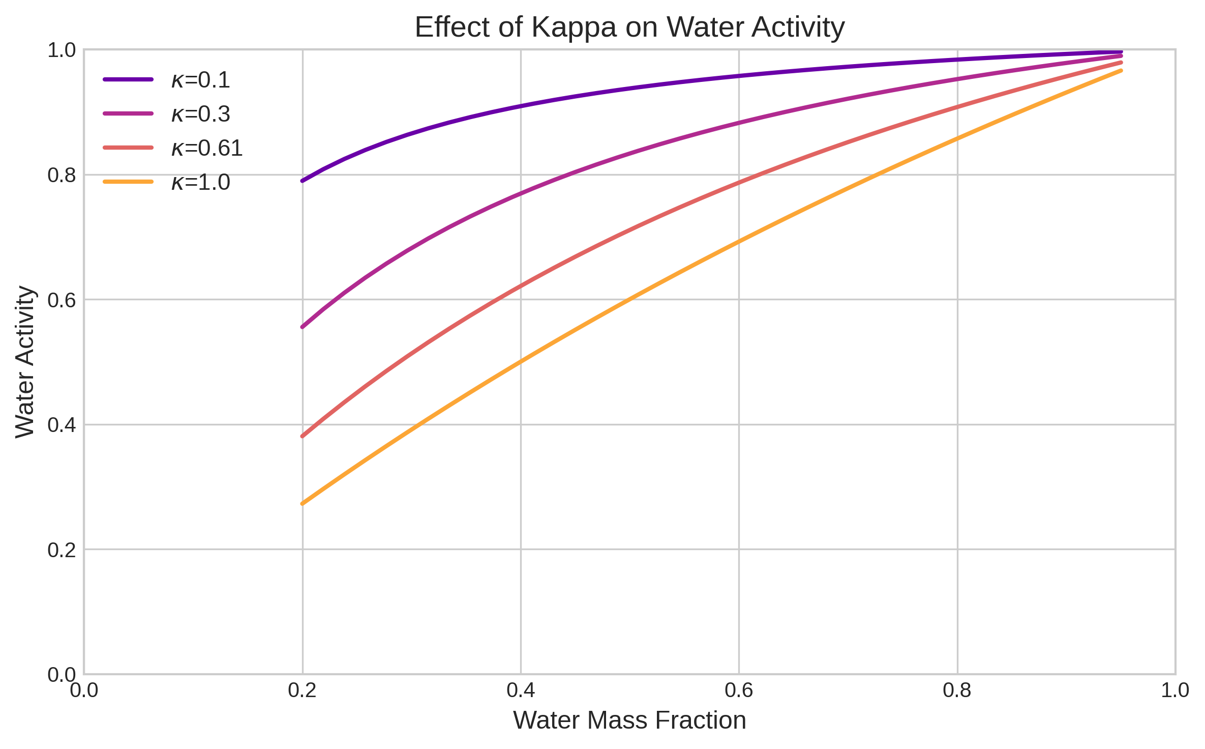
Connect thermodynamics to a partitioning endpoint
Section titled “Connect thermodynamics to a partitioning endpoint”The final calculation prescribes water activity 0.75 in a liquid–vapor partitioning model. Interpreting a_w as relative humidity requires equilibrium and neglect of curvature. This solver does not advance a particle population or determine a time to equilibrium.
Python · section 13
# Create partitioning strategy at 75% RHpartitioning = par.equilibria.LiquidVaporPartitioningStrategy(    water_activity=0.75,)
print(f"Strategy: {type(partitioning).__name__}")print(f"Target water activity: {partitioning.water_activity}")
Strategy: LiquidVaporPartitioningStrategy
Target water activity: 0.75Inspect volatility and concentration scales
Section titled “Inspect volatility and concentration scales”The three dry C* values, 10⁻⁶–10⁻² µg m⁻³, are small relative to the total organic inputs of 1, 5, and 10 µg m⁻³. Near-complete condensation is therefore expected for this example. This interface uses g mol⁻¹ for molar mass. Read the partition coefficients together with water content and the numerical residual, rather than interpreting solver return as physical validation.
Python · section 14
# Define organic species (3 volatility classes)c_star_j_dry = np.array([1e-6, 1e-4, 1e-2])  # saturation conc (ug/m^3)concentration_organic = np.array([1.0, 5.0, 10.0])  # ug/m^3molar_mass = np.array([200.0, 200.0, 200.0])  # g/molo2c_ratio = np.array([0.2, 0.3, 0.5])density = np.array([1200.0, 1200.0, 1200.0])  # kg/m^3
# Solve for equilibriumresult = partitioning.solve(    c_star_j_dry=c_star_j_dry,    concentration_organic_matter=concentration_organic,    molar_mass=molar_mass,    oxygen2carbon=o2c_ratio,    density=density,)
print("=== Equilibrium Results ===")print(f"Partition coefficients: {result.partition_coefficients}")print(f"Alpha phase water: {result.alpha_phase.water_concentration:.2f} ug/m^3")print(f"Optimization error: {result.error:.2e}")
=== Equilibrium Results ===
Partition coefficients: [0.99999998 0.99999838 0.9998916 ]
Alpha phase water: 4.51 ug/m^3
Optimization error: 5.57e-14Separate changes in water from changes in organic mass
Section titled “Separate changes in water from changes in organic mass”The left panel shows an unweighted mean of species partition coefficients; it is not the loading-weighted condensed organic fraction. The right panel shows alpha-phase water only. Because organic partitioning is already near one, a small vertical range on the left can exaggerate its visual importance relative to the water change. These prescribed-activity endpoints are not a single time-dependent humidification experiment.
Python · section 15
# Calculate partitioning at different RH valuesrh_values = np.linspace(0.3, 0.95, 20)mean_partitions = []water_contents = []
for rh in rh_values:    strat = par.equilibria.LiquidVaporPartitioningStrategy(water_activity=rh)    res = strat.solve(        c_star_j_dry=c_star_j_dry,        concentration_organic_matter=concentration_organic,        molar_mass=molar_mass,        oxygen2carbon=o2c_ratio,        density=density,    )    mean_partitions.append(np.mean(res.partition_coefficients))    water_contents.append(res.alpha_phase.water_concentration)
# Plotfig, (ax1, ax2) = plt.subplots(1, 2, figsize=(12, 4.5))
ax1.plot(rh_values * 100, mean_partitions, "b-", linewidth=2)ax1.set_xlabel("Relative Humidity (%)", fontsize=12)ax1.set_ylabel("Mean Partition Coefficient", fontsize=12)ax1.set_title("Partitioning vs RH", fontsize=14)ax1.set_xlim(30, 100)
ax2.plot(rh_values * 100, water_contents, "g-", linewidth=2)ax2.set_xlabel("Relative Humidity (%)", fontsize=12)ax2.set_ylabel("Water Content ($\\mu$g/m$^3$)", fontsize=12)ax2.set_title("Water Uptake vs RH", fontsize=14)ax2.set_xlim(30, 100)
plt.tight_layout()plt.show()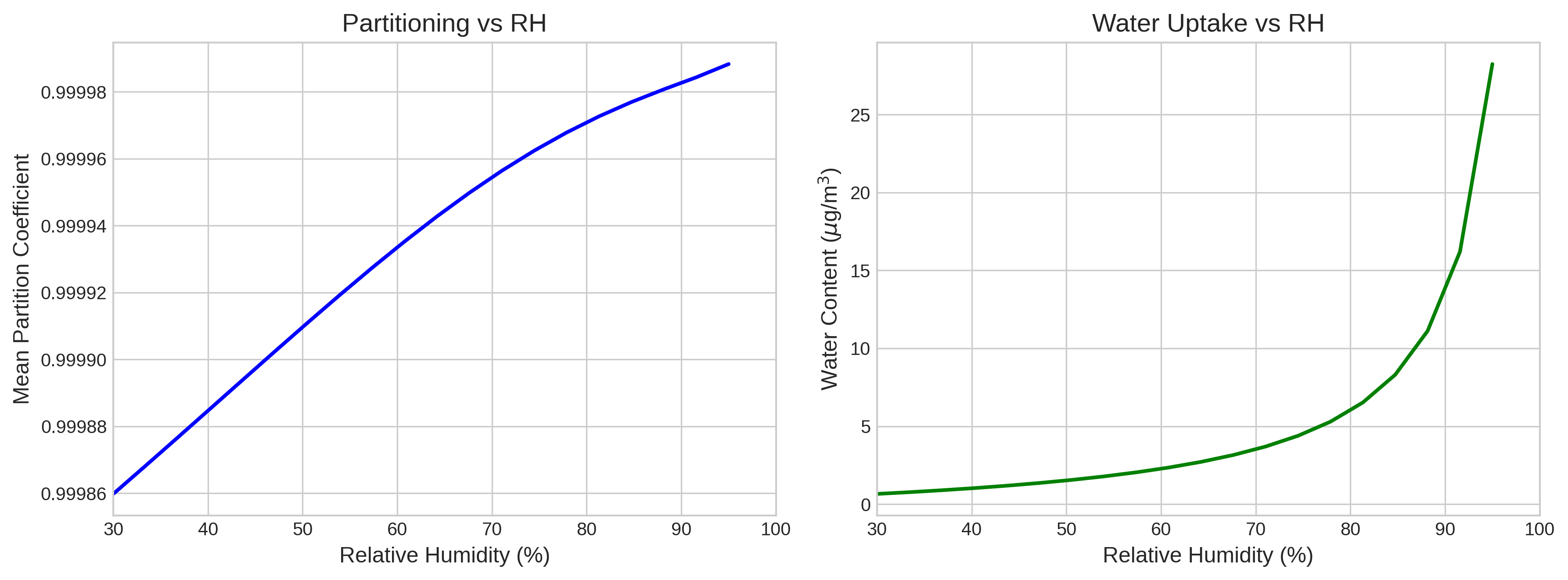
Build a comparison that answers your question
Section titled “Build a comparison that answers your question”This sequence shows why activity-model choice, composition coordinate, and output species must be explicit. Ideal mole fractions provide a checkable reference; BAT and κ encode additional assumptions for different applications. The partitioning example demonstrates that substantial water changes can coexist with nearly unchanged condensed organic fractions.
For your study, choose one observable—equilibrium pressure, water growth factor, or condensed organic mass—and compare models with matched inputs. Check the model domain, numerical residuals, and material accounting, then seek an independent reference. If timescale matters, connect the endpoint to a condensation trajectory with the same reservoir and surface assumptions.
See activity theory, phase-equilibrium theory, and the supported activity interfaces for the equations and implementation contracts.
Explore this topic: Chemical activity