

Direct CUDA nucleation with explicit species mapping
Direct CUDA nucleation with explicit species mapping
Section titled “Direct CUDA nucleation with explicit species mapping”Why does a larger simulated volume create more particles without changing the formation rate per cubic metre? This deliberately tiny example separates unit events, represented counts, and gas mass density. Read CPU nucleation for the source law before following explicit device storage and species binding.
Map precursor gas to particle material and inject unit-count neutral
particles into free slots. Counts and gas density use different units.
Run this script with --cuda to reproduce the published figures.
The unflagged command retains its portable Warp CPU regression.
Python · section 1
"""Run the bounded direct-Warp nucleation step with explicit transfers.
The package-exported ``nucleation_step_gpu`` is used for execution, whileconfiguration and sidecar records are imported from their concrete modules.Warp is required; this example intentionally has no CPU-physics fallback."""
import numpy as npimport numpy.testing as nptimport warp as wpfrom particula.dynamics.nucleation.species_mapping import NucleationSpeciesMapfrom particula.gas import EnvironmentData, GasDatafrom particula.gpu import (    from_warp_environment_data,    from_warp_gas_data,    from_warp_particle_data,    to_warp_environment_data,    to_warp_gas_data,    to_warp_particle_data,)from particula.gpu.kernels import nucleation_step_gpufrom particula.gpu.kernels.exhaustion import ResamplingBuffersfrom particula.gpu.kernels.nucleation import (    NucleationConfig,    NucleationDiagnosticBuffers,    NucleationExhaustionBuffers,    NucleationExhaustionControls,    NucleationFinalizedDemandBuffers,    NucleationScratchBuffers,)from particula.gpu.nucleation_species_mapping import (    prepare_nucleation_species_map,)from particula.particles import ParticleDatafrom particula.util.constants import AVOGADRO_NUMBER

def _buffers(    device: str,) -> tuple[    NucleationScratchBuffers,    NucleationFinalizedDemandBuffers,    NucleationDiagnosticBuffers,    NucleationExhaustionBuffers,]:    """Allocate caller-owned sidecars for the B=1, N=2, S=1 fixture.
    Args:        device: Warp device that owns every allocated sidecar.
    Returns:        Scratch, finalized-demand, diagnostic, and exhaustion sidecars on        ``device``.    """
    def f64(shape: tuple[int, ...]) -> object:        """Allocate a float64 sidecar on the selected Warp device.
        Args:            shape: Dimensions of the sidecar.
        Returns:            A zero-initialized Warp float64 array.        """        return wp.zeros(shape, dtype=wp.float64, device=device)
    def ones(shape: tuple[int, ...]) -> object:        """Allocate a float64 sidecar initialized to one.
        Args:            shape: Dimensions of the sidecar.
        Returns:            A one-initialized Warp float64 array.        """        return wp.ones(shape, dtype=wp.float64, device=device)
    def i32(shape: tuple[int, ...]) -> object:        """Allocate an int32 sidecar on the selected Warp device.
        Args:            shape: Dimensions of the sidecar.
        Returns:            A zero-initialized Warp int32 array.        """        return wp.zeros(shape, dtype=wp.int32, device=device)
    resampling = ResamplingBuffers(        i32((1,)),        i32((1,)),        i32((1, 2)),        i32((1, 2)),        i32((1, 2)),        f64((1, 2, 1)),        f64((1, 2)),        f64((1, 2)),        f64((1, 2)),        f64((1,)),        f64((1,)),        f64((1,)),        f64((1,)),        i32((1,)),    )    return (        NucleationScratchBuffers(f64((1,)), f64((1,)), f64((1,))),        NucleationFinalizedDemandBuffers(i32((1,)), f64((1,)), f64((1, 1))),        NucleationDiagnosticBuffers(            i32((1,)), i32((1, 2)), i32((1, 2)), i32((1,)), i32((1,))        ),        NucleationExhaustionBuffers(            resampling,            f64((1,)),            f64((1,)),            ones((1,)),            ones((1,)),            ones((1,)),            f64((1,)),            i32((1,)),            i32((1,)),            i32((1,)),            i32((1,)),            i32((1, 2)),        ),    )

def run_example(    volume: float = 1.0,    *,    device: str = "cpu",) -> tuple[ParticleData, GasData, EnvironmentData]:    """Run one deterministic nucleation event on the selected Warp device.
    Args:        volume: Represented volume in m³. Particle concentration stores counts;            gas concentration stores kg/m³. The two slots accommodate the            default one-event demonstration and its two-m³ regression case.        device: Explicit Warp device; defaults to CPU. CUDA never falls back.
    Returns:        Restored CPU particle, gas, and environment data after synchronization.    """    particles = ParticleData(        masses=np.zeros((1, 2, 1), dtype=np.float64),        concentration=np.zeros((1, 2), dtype=np.float64),        charge=np.zeros((1, 2), dtype=np.float64),        density=np.array([1000.0], dtype=np.float64),        volume=np.array([volume], dtype=np.float64),        distribution_type="particle_resolved",    )    gas = GasData(        name=["precursor"],        molar_mass=np.array([0.1]),        concentration=np.array([[1.0]], dtype=np.float64),        partitioning=np.array([True]),    )    environment = EnvironmentData(        temperature=np.array([300.0]),        pressure=np.array([101325.0]),        saturation_ratio=np.array([[1.0]]),    )    initial_inventory = gas.concentration * particles.volume[:, None]    gpu_particles = to_warp_particle_data(particles, device=device)    gpu_gas = to_warp_gas_data(gas, device=device)    gpu_environment = to_warp_environment_data(environment, device=device)    # Names remain host-owned; upload explicit configuration for these exact    # carriers after transfer. Equal species widths do not define a mapping.    species_binding = prepare_nucleation_species_map(        gpu_particles,        gpu_gas,        gas_names=gas.name,        species_map=NucleationSpeciesMap(tuple(gas.name), ((0, 0),)),    )    scratch, finalized, diagnostics, exhaustion = _buffers(device)    config = NucleationConfig(        rate_law="activation",        coefficient=0.1 / AVOGADRO_NUMBER,        survival_factor=1.0,        precursor_index=0,        molecule_counts=(1,),        formation_diameter=1.0e-9,        precursor_number_concentration_lower=0.0,        precursor_number_concentration_upper=1.0e30,        temperature_lower=200.0,        temperature_upper=400.0,    )    returned_particles, returned_gas = nucleation_step_gpu(        gpu_particles,        gpu_gas,        config,        1.0,        environment=gpu_environment,        species_binding=species_binding,        scratch=scratch,        finalized_demand=finalized,        diagnostics=diagnostics,        exhaustion_controls=NucleationExhaustionControls(False, False),        exhaustion_buffers=exhaustion,    )    assert returned_particles is gpu_particles and returned_gas is gpu_gas    wp.synchronize()    restored_particles = from_warp_particle_data(gpu_particles, sync=False)    restored_gas = from_warp_gas_data(gpu_gas, name=gas.name, sync=False)    restored_environment = from_warp_environment_data(        gpu_environment,        sync=False,    )    assert restored_particles.masses.shape == (1, 2, 1)    assert restored_gas.concentration.shape == (1, 1)    assert int(np.count_nonzero(restored_particles.concentration)) > 0    assert restored_gas.concentration[0, 0] <= gas.concentration[0, 0]    particle_inventory = np.sum(        restored_particles.masses        * restored_particles.concentration[:, :, None],        axis=1,    )    npt.assert_allclose(        particle_inventory        + restored_gas.concentration * restored_particles.volume[:, None],        initial_inventory,        rtol=1e-12,        atol=1e-30,    )    return restored_particles, restored_gas, restored_environment
Separate represented counts from number density
Section titled “Separate represented counts from number density”Doubling represented volume doubles the number of unit events at the same formation rate per cubic metre. Each injected particle consumes one precursor molecule. Two free slots suffice for this deliberately small demonstration; the prepared lifecycle tutorial uses thousands of boxes and an active pulse.
Python · section 2
def run_publication():    """Require CUDA and compare one- and two-cubic-metre source events."""    import matplotlib.pyplot as plt
    if not wp.is_cuda_available():        raise RuntimeError("This publication run requires CUDA")    results = [run_example(volume=v, device="cuda:0") for v in (1.0, 2.0)]    count = np.array([p.concentration.sum() for p, _, _ in results])    volumes = np.array([1.0, 2.0])    npt.assert_array_equal(count, volumes)    fig, axes = plt.subplots(1, 2, figsize=(8, 3.5), constrained_layout=True)    axes[0].bar(volumes, count, color="#287a90", width=0.6)    axes[0].set(        xlabel="Represented volume (m³)",        ylabel="Injected count",        xticks=volumes,        yticks=[0, 1, 2],    )    axes[1].bar(volumes, count / volumes, color="#be6c39", width=0.6)    axes[1].set(        xlabel="Represented volume (m³)",        ylabel="Injected number density (m$^{-3}$)",        xticks=volumes,    )    fig.suptitle("Unit-event nucleation · " + wp.get_device("cuda:0").name)    print("Counts:", count, "Number densities (m^-3):", count / volumes)    print("Per-species particle + gas inventory checks passed.")    plt.show()    return results

if __name__ == "__main__":    import sys
    if "--cuda" in sys.argv[1:]:        run_publication()    else:        run_example()        print("Direct Warp nucleation example completed on device=cpu.")
Explicit cuda invocation
result = run_publication()Warp 1.11.1 initialized:
CUDA Toolkit 12.9, Driver 13.4
Devices:
"cpu" : "CPU"
"cuda:0" : "NVIDIA GeForce RTX 5060" (8 GiB, sm_120, mempool enabled)
Kernel cache:
~/.cache/warp/1.11.1
Module particula.gpu.kernels.nucleation 1124f09 load on device 'cuda:0' took 2.53 ms (cached)
Module particula.gpu.kernels._population_validation 65eaa49 load on device 'cuda:0' took 0.49 ms (cached)
Module particula.gpu.kernels.slot_management 0375e2c load on device 'cuda:0' took 0.57 ms (cached)
Module particula.gpu.kernels.exhaustion ccbadfa load on device 'cuda:0' took 1.77 ms (cached)
Counts: [1. 2.] Number densities (m^-3): [1. 1.]
Per-species particle + gas inventory checks passed.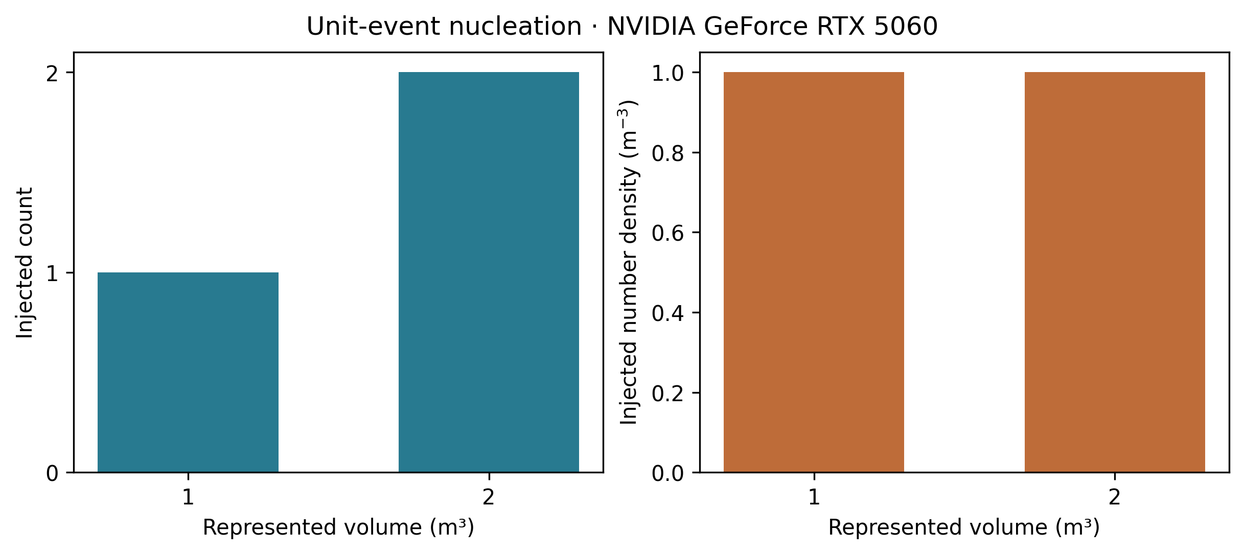
Read the two bars together
Section titled “Read the two bars together”The 1 and 2 m³ cases inject one and two unit-count particles, respectively; both give 1 m⁻³ after the one-second update. The coefficient and 1 kg m⁻³ gas reservoir are chosen for this count-scaling demonstration. One precursor molecule per nucleus is bookkeeping here, not a validated nanoparticle formation model. The configuration’s formation diameter should not be read as a measured output size; material mass and density determine the represented particle radius.
Each injected molecule is tiny compared with that reservoir. The aggregate inventory tolerance alone cannot resolve its depletion, so do not use this case as strong evidence of small gas-consumption accuracy. For a nucleation study, choose a defensible rate and nucleus composition, compare event demand with available gas and free slots, and test per-species source accounting at a resolvable scale. The prepared lifecycle adds active source pulses to an evolving population.
Explore this topic: Direct kernels