

From one sphere to a cloud's optical signal
From one sphere to a cloud’s optical signal
Section titled “From one sphere to a cloud’s optical signal”How can particle size and concentration become a spectrum, a polarization signature, or an attenuated light beam? This CPU example connects three levels: single-particle cross sections, angle-dependent scattering, and population extinction integrated over a path. They answer different observational questions; one bulk extinction number cannot recover all the angular information.
The calculation uses homogeneous independent spheres in a nonabsorbing medium, with radius and vacuum wavelength in metres and angles in radians. The constant complex refractive indices are illustrative, not measured spectral material data. See the optics guide for conventions and exclusions. The calculation changes no particle mass, temperature, or gas composition.
Python · section 1
import matplotlib.pyplot as pltimport numpy as npfrom particula.optics import ( apply_mueller_matrix, get_column_optics, get_cross_sections, get_differential_cross_sections, get_mie_coefficients, get_mie_efficiencies, get_mueller_matrix, get_population_optics, get_population_weights, get_scattering_amplitudes,)Connect particle, population, and path calculations
Section titled “Connect particle, population, and path calculations”simulate() first converts Mie efficiencies into cross sections and checks
extinction closure. It then calculates angular amplitudes and applies the
Mueller matrix to unpolarized light. Finally it weights droplet cross sections
by number density and integrates extinction through a uniform column.
The count-to-density equality and τ=extinction×length assertion check two
places where otherwise plausible unit mistakes would alter the result.
plot_results() renders the compact observations; it does not rerun the physics.
Python · section 2
def simulate():    """Calculate compact spectral, angular and column observations."""    wavelength = np.linspace(400e-9, 1000e-9, 121)    radius = 200e-9    efficiency = get_mie_efficiencies(radius, wavelength, 1.5 + 0.02j)    cross = get_cross_sections(efficiency, radius)    np.testing.assert_allclose(        cross.extinction, cross.scattering + cross.absorption, rtol=1e-12    )
    angle = np.linspace(0, np.pi, 361)    angular_wave = 550e-9    angular_radius = 500e-9    coefficients = get_mie_coefficients(        1.33 + 1e-8j, 2 * np.pi * angular_radius / angular_wave    )    amplitudes = get_scattering_amplitudes(coefficients, angle)    differential = get_differential_cross_sections(*amplitudes, angular_wave)    scattered = apply_mueller_matrix(        get_mueller_matrix(*amplitudes), [1.0, 0.0, 0.0, 0.0]    )    polarization = -scattered[:, 1] / scattered[:, 0]    assert np.all(abs(polarization) <= 1 + 1e-12)
    # Explicit discrete bin densities: normalized lognormal weights per bin.    cloud_radius = np.geomspace(1e-6, 30e-6, 64)    bin_shape = np.exp(-0.5 * (np.log(cloud_radius / 8e-6) / 0.35) ** 2)    number_density = 1e8 * bin_shape / bin_shape.sum()  # particles / m³    cloud_q = get_mie_efficiencies(cloud_radius, 550e-9, 1.33 + 1e-8j)    cloud_cross = get_cross_sections(cloud_q, cloud_radius)    bulk = get_population_optics(cloud_cross, cloud_q.asymmetry, number_density)    # Represented counts / representative volume give the same optical field.    volume = 2e-6  # m³; this does not define an optical path length.    resolved = get_population_weights(        number_density * volume, "particle_resolved", volume=volume    )    np.testing.assert_allclose(resolved, number_density, rtol=1e-14)    path_length = np.linspace(0, 500, 101)    columns = get_column_optics(        np.full((len(path_length), 1), bulk.extinction),        path_length[:, None],    )    np.testing.assert_allclose(        columns.optical_depth, bulk.extinction * path_length, rtol=1e-14    )    assert columns.transmission[0] == 1    assert np.all(np.diff(columns.transmission) <= 0)    return {        "wavelength_nm": (wavelength * 1e9).tolist(),        "cross_sections_m2": {            "extinction": cross.extinction.tolist(),            "scattering": cross.scattering.tolist(),            "absorption": cross.absorption.tolist(),        },        "angle_degrees": np.rad2deg(angle).tolist(),        "differential_m2_sr": {            "perpendicular": differential.perpendicular.tolist(),            "parallel": differential.parallel.tolist(),            "unpolarized": differential.unpolarized.tolist(),        },        "linear_polarization": polarization.tolist(),        "path_length_m": path_length.tolist(),        "optical_depth": columns.optical_depth.tolist(),        "transmission": columns.transmission.tolist(),        "cloud_extinction_m_inv": float(bulk.extinction),        "cloud_single_scattering_albedo": float(bulk.single_scattering_albedo),        "cloud_asymmetry": float(bulk.asymmetry),    }

def plot_results(report):    """Render compact saved optical observations without rerunning physics."""    fig, ax = plt.subplots(figsize=(7, 4), constrained_layout=True)    for label, values in report["cross_sections_m2"].items():        ax.plot(report["wavelength_nm"], np.array(values) * 1e12, label=label)    ax.set(        xlabel="Vacuum wavelength [nm]",        ylabel="Cross section [µm²]",        title="200 nm radius sphere · illustrative index 1.5 + 0.02i",    )    ax.legend()    ax.grid(alpha=0.2)
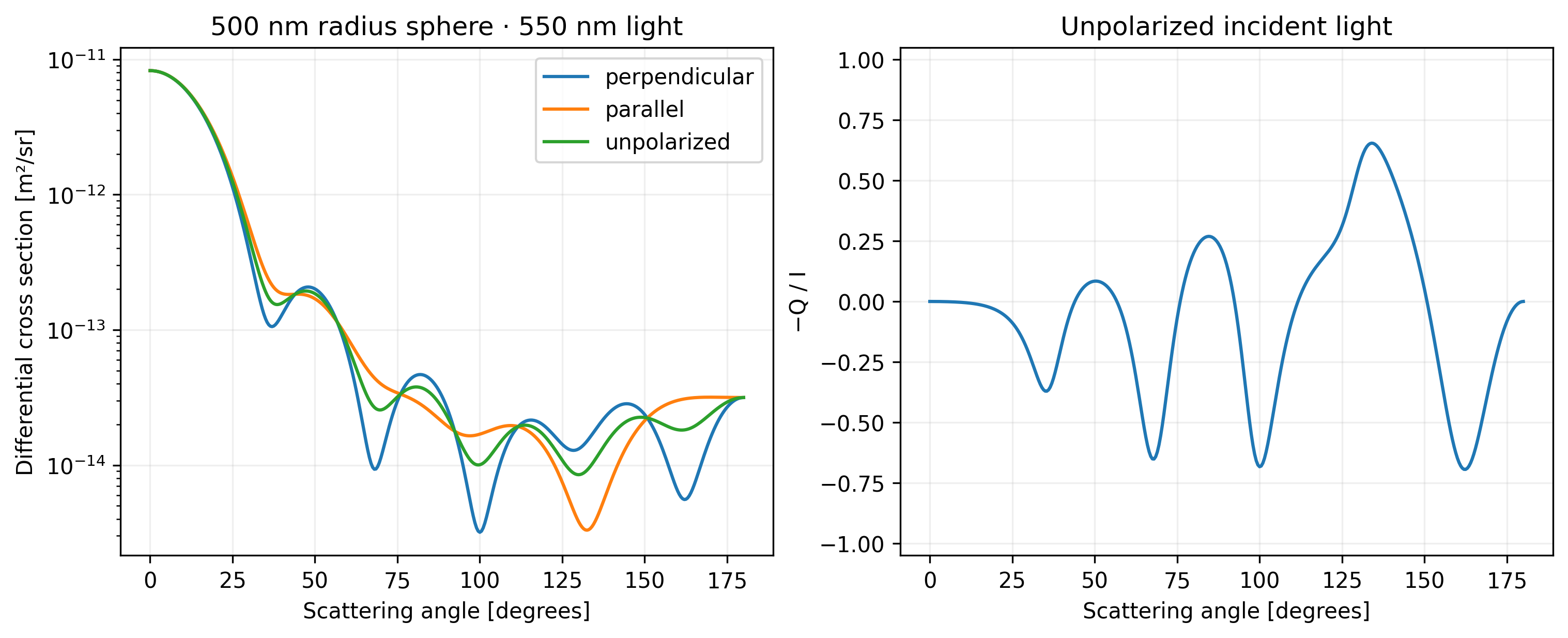
    fig, axes = plt.subplots(1, 2, figsize=(10, 4), constrained_layout=True)    for label, values in report["differential_m2_sr"].items():        axes[0].semilogy(report["angle_degrees"], values, label=label)    axes[0].set(        xlabel="Scattering angle [degrees]",        ylabel="Differential cross section [m²/sr]",        title="500 nm radius sphere · 550 nm light",    )    axes[0].legend()    axes[1].plot(report["angle_degrees"], report["linear_polarization"])    axes[1].set(        xlabel="Scattering angle [degrees]",        ylabel="−Q / I",        ylim=(-1.05, 1.05),        title="Unpolarized incident light",    )    for ax in axes:        ax.grid(alpha=0.2)
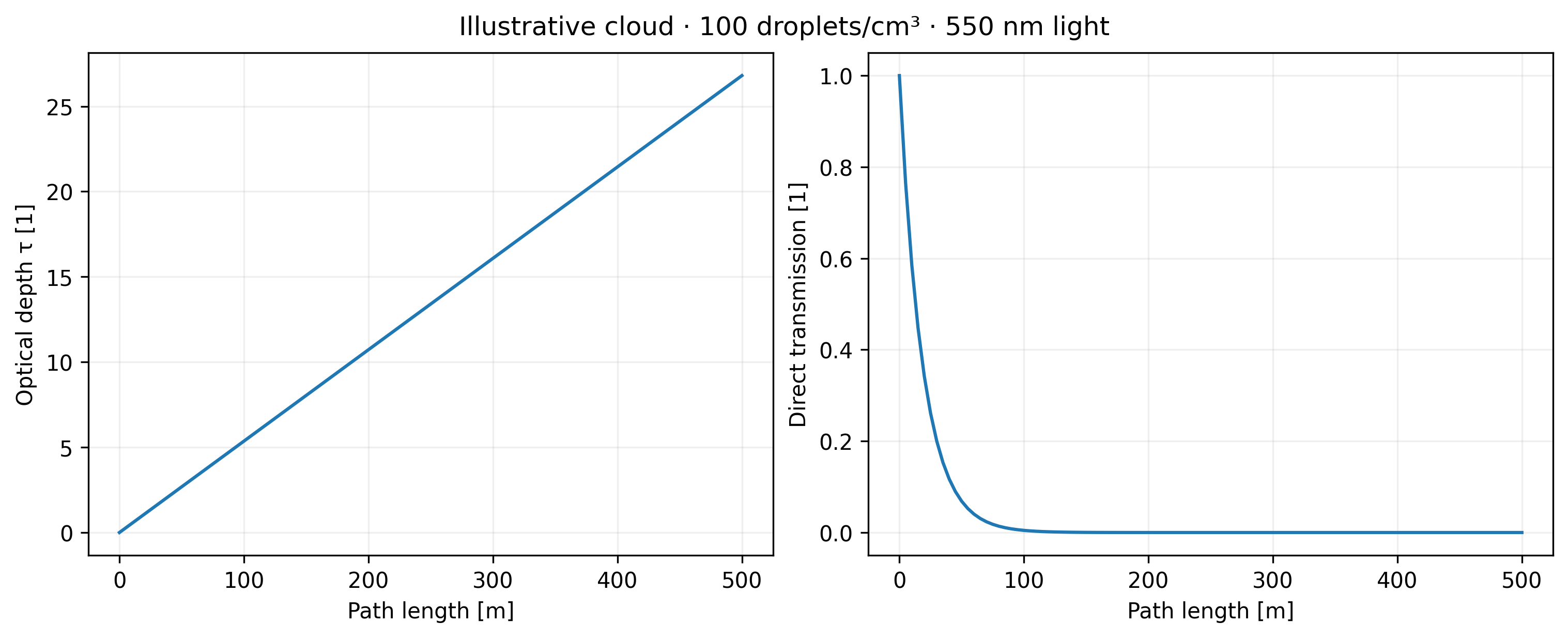
    fig, axes = plt.subplots(1, 2, figsize=(10, 4), constrained_layout=True)    for ax, key, label in zip(        axes,        ["optical_depth", "transmission"],        ["Optical depth τ [1]", "Direct transmission [1]"],        strict=True,    ):        ax.plot(report["path_length_m"], report[key])        ax.set(xlabel="Path length [m]", ylabel=label)        ax.grid(alpha=0.2)    fig.suptitle("Illustrative cloud · 100 droplets/cm³ · 550 nm light")    print(f"Cloud extinction: {report['cloud_extinction_m_inv']:.6g} m⁻¹")    print(        f"Single-scattering albedo: {report['cloud_single_scattering_albedo']:.8f}"    )    print(f"Scattering-weighted g: {report['cloud_asymmetry']:.6f}")    return report

def run_example():    """Calculate once and plot the resulting optical observations."""    return plot_results(simulate())
Read the three optical observations together
Section titled “Read the three optical observations together”The first figure uses a 200 nm radius sphere with index 1.5 + 0.02i across 400–1000 nm. Extinction is scattering plus absorption; the assertion checks that identity. Cross sections are areas, not dimensionless efficiencies. The varying spectrum here comes from size parameter, since the refractive index is held fixed. A measured material spectrum could add another dependence.
The second figure changes the particle to a 500 nm radius sphere with index 1.33 + 10⁻⁸i at 550 nm. Differential cross sections describe scattering into a direction, in m²/sr. The adjoining −Q/I curve uses unpolarized incident light and the scattering-plane convention: positive values favor perpendicular linear polarization. Its sign and angular structure contain information absent from a total cross section; the magnitude check enforces a basic bound.
The third figure sums a discrete lognormal-shaped set of 64 radius bins from 1–30 µm at a total 10⁸ particles/m³ (100/cm³). These weights are number per bin per volume, not dN/dr. The recorded extinction is about 0.0536 m⁻¹ and the scattering-weighted asymmetry is about 0.866. Optical depth grows linearly with path length; direct-beam transmission falls as exp(−τ). The 2×10⁻⁶ m³ representative volume used in the count conversion is not a light-path length.
A nearly unit single-scattering albedo means little absorption per extinction event. It does not imply high direct transmission: scattering also removes photons from the unscattered beam. Diffuse radiation and multiple scattering are outside this calculation.
Python · section 3
if __name__ == "__main__": result = run_example() plt.show()Explicit cpu invocation
result = run_example()Cloud extinction: 0.0535973 m⁻¹
Single-scattering albedo: 0.99999775
Scattering-weighted g: 0.865576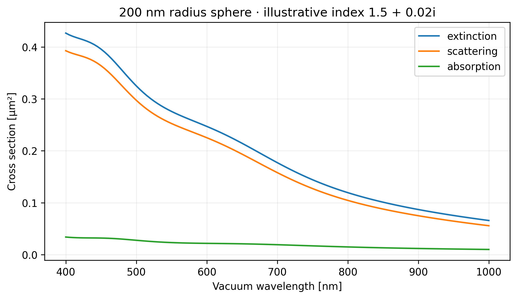
Adapt the observation to your research question
Section titled “Adapt the observation to your research question”A sphere’s optical response can be aggregated into a population signal only after specifying the number-density measure, and into transmission only after specifying the path. Keeping those choices explicit prevents confusing a sample volume with a viewing geometry.
To investigate whether an observed extinction change comes from particle number or size, vary those inputs separately and compare both extinction and angular polarization. Use measured wavelength-dependent indices before identifying a material. The absorption spectrum could also feed a heating calculation, but that extension needs incident irradiance, thermal properties, emission and an energy balance; evaporation additionally needs mass transfer and latent heat. For large batches, the CUDA optics example tests the same optical quantities against CPU calculations.
Explore this topic: Optical properties