

Distinguish chemical conversion from a timed emission and dilution
Distinguish chemical conversion from a timed emission and dilution
Section titled “Distinguish chemical conversion from a timed emission and dilution”A concentration can change because material reacts, enters the box, or leaves it. This CPU example composes all three mechanisms and compares the trajectory with an analytic reference. You can use it as a template for checking timed custom chemistry before introducing a more complicated reaction system.
A and B have equal molar masses and undergo first-order A → B conversion at 0.3 s⁻¹. Dilution removes both at 0.05 s⁻¹. At 4 s, a pulse adds A to two independent boxes of volumes 1 and 2 m³; there is no exchange between boxes. Their different temperatures are stored state, but this constant-rate chemistry does not use temperature to change its coefficient.
Gas concentration is kg m⁻³, particle weights are represented counts, volume is m³, and time is s. The dilution reference provides the simplest limiting case. Here 0.5 s outer steps each contain two substeps, and the pulse is deliberately aligned with a substep boundary.
Python · section 1
"""Timed public CPU process composition with a SciPy analytical check."""
import matplotlib.pyplot as pltimport numpy as npfrom particula import Aerosol, BoxProcess, FieldSpec, FunctionProcessfrom particula.dynamics import Dilution, DilutionStrategyfrom particula.gas import EnvironmentData, GasDatafrom particula.particles import ParticleDatafrom scipy.integrate import solve_ivp

class Chemistry(BoxProcess):    """Convert A into equal-molar-mass B with a first-order rate [s^-1]."""
    def __init__(self, rate=0.3):        """Declare immutable configuration and the sole permitted destination."""        if not np.isfinite(rate) or rate < 0:            raise ValueError("rate must be finite and nonnegative")        super().__init__(            name="chemistry",            extension_id="example.first_order_chemistry",            reads=("gas.concentration",),            writes=("gas.concentration",),            parameters=(float(rate),),        )        self.rate = float(rate)
    def validate(self, aerosol):        """Require ordered species and equal reactant/product molar masses."""        if aerosol.gas.name != ["A", "B", "inert"]:            raise ValueError("chemistry requires gas order A, B, inert")        if aerosol.gas.molar_mass[0] != aerosol.gas.molar_mass[1]:            raise ValueError("this example requires equal molar masses")
    def advance(self, aerosol, *, time, time_step, context):        """Use arbitrary scientific Python on ordinary one-box native arrays."""        gas = aerosol.gas.concentration
        def reaction(_time, values):            flux = self.rate * values[0]            return (-flux, flux)
        solution = solve_ivp(            reaction,            (time, time + time_step),            gas[0, :2],            rtol=1e-11,            atol=1e-22,        )        if not solution.success:            raise RuntimeError(solution.message)        candidate = solution.y[:, -1]        np.testing.assert_allclose(            candidate.sum(), gas[0, :2].sum(), rtol=1e-12, atol=1e-22        )        gas[0, :2] = candidate
Publish a custom update only after each box succeeds
Section titled “Publish a custom update only after each box succeeds”Each callback receives a detached box with ordinary particle, gas, environment,
and registered-field containers. It edits declared arrays in place and returns
None. Particula checks shapes, identities, declared writes, and valid values
before publishing after all boxes succeed; the callback still owns scientific
accounting. External side effects are not undone by an array rollback.
Species order, shapes, and capacity stay fixed. Chemistry.validate also requires
equal reactant/product molar masses so the simple mass-based A → B transfer is
consistent. More general chemistry would need explicit stoichiometry and units.
The registered field demo.injected records cumulative external mass in kg.
It is an accounting ledger, not a gas concentration subject to dilution. The
scheduled emission rejects a step that crosses the pulse time without starting
there, making a timing error visible rather than smearing the pulse.
Python · section 2
def build_aerosol():    """Construct two independent boxes with different volumes and gas loads."""    aerosol = Aerosol(        particles=ParticleData(            masses=np.full((2, 1, 1), 1e-18),            concentration=np.ones((2, 1)),            charge=np.zeros((2, 1)),            density=np.array([1000.0]),            volume=np.array([1.0, 2.0]),            distribution_type="particle_resolved",        ),        gas=GasData(            name=["A", "B", "inert"],            molar_mass=np.array([0.1, 0.1, 0.029]),            concentration=np.array([[2e-9, 0.0, 1e-6], [5e-9, 0.0, 1e-6]]),            partitioning=np.zeros(3, dtype=bool),        ),        environment=EnvironmentData(            temperature=np.array([298.15, 288.15]),            pressure=np.full(2, 101325.0),            saturation_ratio=np.zeros((2, 3)),        ),    )    aerosol.fields.add(FieldSpec("demo.injected", ("box",), "kg", minimum=0))    return aerosol

def simulate():    """Check every observation against the exact pulse/decay solution."""    aerosol = build_aerosol()    initial = aerosol.gas.concentration.copy()    volume = aerosol.particles.volume.copy()    pulse_time, rate, dilution = 4.0, 0.3, 0.05    pulse = np.array([3e-9, 1e-9])
    def emit(box, *, time, time_step, context):        if time <= pulse_time < time + time_step:            # This schedule is deliberately aligned with the substep grid.            if time != pulse_time:                raise ValueError("split the timestep at the emission boundary")            amount = pulse[int(context.box_id)]            box.gas.concentration[0, 0] += amount            box.fields["demo.injected"][:] += amount * box.particles.volume
    emissions = FunctionProcess(        emit,        name="emissions",        reads=("particles.volume",),        writes=("gas.concentration", "demo.injected"),        parameters=(pulse_time, tuple(float(value) for value in pulse)),    )    processes = (        emissions | Chemistry(rate) | Dilution(DilutionStrategy(dilution))    )    times = np.arange(41) * 0.5    concentrations = [initial.copy()]    for start in times[:-1]:        # Repeated calls supply absolute start time; both substeps share the        # same physical interval across all processes in the sequence.        processes.execute(aerosol, 0.5, sub_steps=2, time=float(start))        concentrations.append(aerosol.gas.concentration.copy())    values = np.asarray(concentrations)    t = times[:, None]    emitted = np.where(t > pulse_time, pulse, 0.0)    total = initial[:, 0] * np.exp(-dilution * t) + emitted * np.exp(        -dilution * (t - pulse_time)    )    reference_a = initial[:, 0] * np.exp(        -(rate + dilution) * t    ) + emitted * np.exp(-(rate + dilution) * (t - pulse_time))    reference = np.stack((reference_a, total - reference_a), axis=2)    np.testing.assert_allclose(        values[:, :, :2], reference, rtol=2e-9, atol=1e-20    )    np.testing.assert_allclose(        values[:, :, 2], initial[:, 2] * np.exp(-dilution * t), rtol=1e-13    )    np.testing.assert_allclose(aerosol.fields["demo.injected"], pulse * volume)    inventory = values[:, :, :2].sum(axis=2) * volume    np.testing.assert_allclose(        inventory, total * volume, rtol=1e-12, atol=1e-22    )    return dict(        time=times.tolist(),        concentrations=values[:, :, :2].tolist(),        reference=reference.tolist(),        inventory=inventory.tolist(),        reference_inventory=(total * volume).tolist(),        injected=aerosol.fields["demo.injected"].tolist(),    )
Read concentration and extensive mass together
Section titled “Read concentration and extensive mass together”The left panel distinguishes A decay from B production in µg m⁻³; dots show the analytic species reference. The right panel multiplies A+B concentration by each box volume to obtain µg. Reaction conserves A+B, whereas dilution reduces it and the scheduled pulse adds it.
The snapshot labeled 4 s is taken just before the pulse is applied at the start
of the next advance; the first recorded post-pulse state is 4.5 s. This sampling
convention explains why a plotted jump can appear after the forcing timestamp.
run_example invokes the plot only after checking species and inventory.
Python · section 3
def plot_results(report):    """Plot species evolution and independently checked extensive inventories."""    values, reference = (        np.asarray(report["concentrations"]),        np.asarray(report["reference"]),    )    fig, axes = plt.subplots(1, 2, figsize=(11, 4.2), constrained_layout=True)    for box, color in enumerate(("tab:blue", "tab:orange")):        for species, linestyle in enumerate(("-", "--")):            axes[0].plot(                report["time"],                values[:, box, species] * 1e9,                color=color,                ls=linestyle,                label=f"Box {box + 1}, {'AB'[species]}",            )            axes[0].plot(                report["time"][::4],                reference[::4, box, species] * 1e9,                color=color,                marker="o",                ls="none",                ms=3,            )        axes[1].plot(            report["time"],            np.asarray(report["inventory"])[:, box] * 1e9,            color=color,            label=f"Box {box + 1}",        )        axes[1].plot(            report["time"][::4],            np.asarray(report["reference_inventory"])[::4, box] * 1e9,            "o",            color=color,            ms=3,        )    axes[0].set(        ylabel="Gas concentration (µg m⁻³)",        title="SciPy chemistry + native dilution",    )    axes[1].set(ylabel="A + B inventory (µg)", title="External pulse at 4 s")    for ax in axes:        ax.set_xlabel("Time (s)")        ax.legend()        ax.grid(alpha=0.2)    fig.suptitle("Lines: simulation · dots: analytical reference")    plt.show()

def run_example():    """Run the checked calculation and render the saved-data plot."""    report = simulate()    print("Analytical species and inventory checks passed for both boxes.")    print("Injected mass (kg per box):", report["injected"])    plot_results(report)    return report

if __name__ == "__main__":    run_example()
Explicit cpu invocation
report = run_example()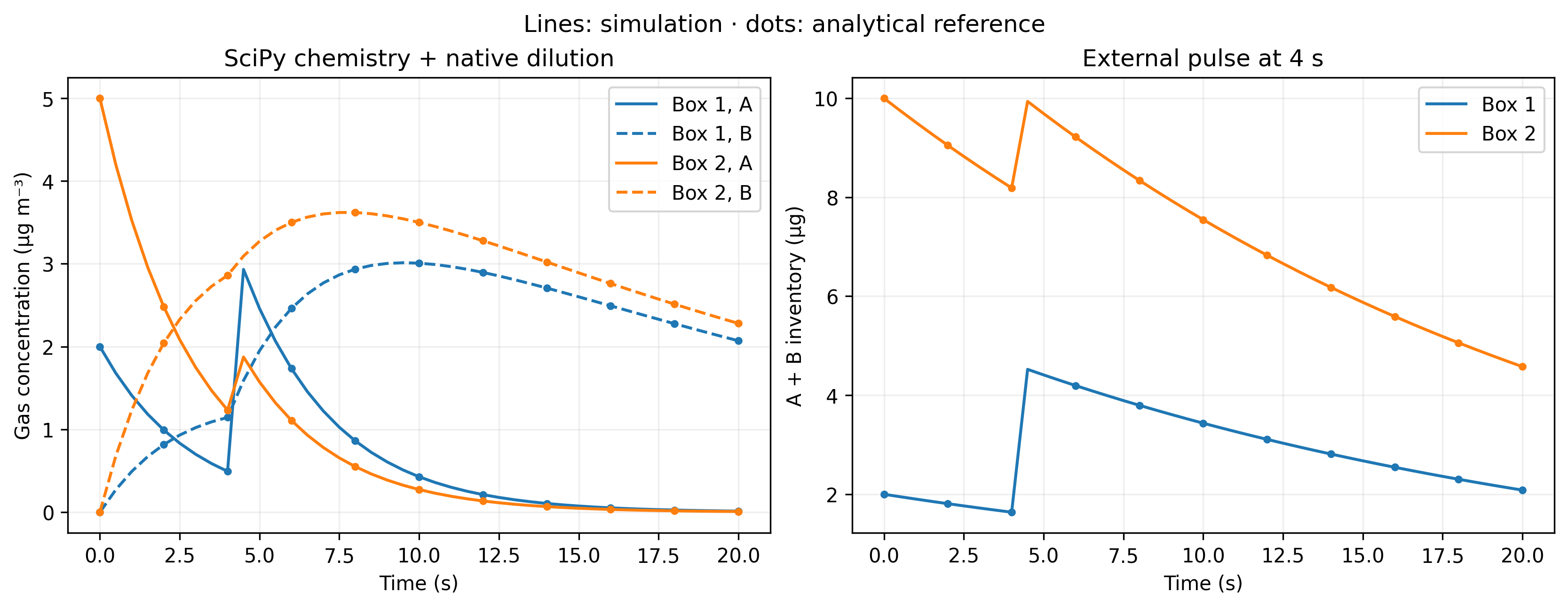
What agreement with the reference means
Section titled “What agreement with the reference means”The species and extensive-inventory assertions compare every recorded state with the closed-form pulse, reaction, and dilution solution. The injected masses are 3×10⁻⁹ and 2×10⁻⁹ kg for the two boxes, despite their respective concentration pulses of 3×10⁻⁹ and 1×10⁻⁹ kg m⁻³. Volume matters when interpreting the budget. The agreement checks this linear reaction and aligned schedule; it does not validate a nonlinear chemical mechanism or arbitrary event timing.
To adapt the pattern to a measured emission history, split steps at every forcing discontinuity and compare cumulative input, chemical transfers, and removals. Then refine timesteps and solver tolerances for the actual mechanism. The custom backend example explains what additional work is needed before assuming a Python callback can run on CUDA.
Explore this topic: Custom processes and fields