

Ionparticle Coagulation
Ion–Particle Coagulation
Section titled “Ion–Particle Coagulation”This notebook investigates the coagulation of positively charged aerosol particles (0 to 11 elementary charges) with negatively charged ions. Specifically, we analyze collisions between a 3 nm radius particle and a 0.45 nm radius ion under various coagulation models.
Coagulation Kernels
Section titled “Coagulation Kernels”To model ion–particle interactions, we compare several coagulation kernels, each incorporating different physical effects:
- Hard Sphere Kernel: Assumes Brownian collisions with idealized electrostatic interactions.
- Dyachkov et al. (2007) Kernel – Physics of Plasmas, 14, 042102
- Gatti & Kortshagen (2008) Kernel – Phys. Rev. E, 78, 046402
- Gopalakrishnan et al. (2012) Kernel – Phys. Rev. E, 85, 026410
- Chahl et al. (2019) Kernel – Aerosol Sci. Technol., 53(8), 933-957
Each kernel accounts for charge-dependent coagulation efficiencies. This study aims to compare these models to evaluate how charge influences ion–particle collision rates.
Python · section 1
# In Colab uncomment the following command to install particula:#!pip install particula[extra] --quietimport numpy as npfrom matplotlib import pyplot as plt
# from particula.util.lf2013_coagulation import lf2013_coag_fullimport particula as parThis block is setting up the properties of a set of aerosol particles, calculating key parameters related to their movement and interaction within a gaseous environment, and determining their diffusion behavior.
1. Environmental Setup
Section titled “1. Environmental Setup”- The temperature is set to 278.0 K, which will be used for further calculations.
2. Particle Properties
Section titled “2. Particle Properties”- Particle Radius: A set of particles is defined with radii ranging from 0.45 nm to 3 nm.
- Charge: The particles have a range of electric charges from -1 to +12.
- Density: The particle density is primarily set to 1700 kg/m³, with one particle (ion) at 1860 kg/m³.
3. Mass Calculation
Section titled “3. Mass Calculation”- Using the formula for the volume of a sphere and the given densities, the mass of each particle is computed.
4. Gas Properties
Section titled “4. Gas Properties”- The dynamic viscosity of the surrounding gas is obtained using the
par.gas.get_dynamic_viscosity()function.
5. Knudsen Number Calculation
Section titled “5. Knudsen Number Calculation”- The Knudsen number, which determines whether the particle behavior is in the free molecular, transition, or continuum regime, is computed using:
- The mean free path of gas molecules (from
par.gas.get_molecule_mean_free_path()). - The particle radius.
- The mean free path of gas molecules (from
6. Friction Factor
Section titled “6. Friction Factor”- The friction factor, which influences the motion and diffusion of the particles, is calculated using:
- Particle radius
- Dynamic viscosity
- Slip correction factor (using
par.particles.get_cunningham_slip_correction()).
7. Coulomb Enhancement Ratio
Section titled “7. Coulomb Enhancement Ratio”- The Coulomb potential ratio, which determines how electrostatic forces influence particle interactions, is computed using:
- Particle radius
- Charge
- Temperature
8. Diffusive Knudsen Number
Section titled “8. Diffusive Knudsen Number”- Finally, the diffusive Knudsen number, which governs diffusion behavior, is computed using:
- Particle radius
- Particle mass
- Friction factor
- Coulomb potential ratio
- Temperature
Python · section 2
# environmenttemperature = 278.0pressure = 101325.0
# get each particle propertiesparticle_radius = np.array(    [        0.45e-9,        3e-9,        3e-9,        3e-9,        3e-9,        3e-9,        3e-9,        3e-9,        3e-9,        3e-9,        3e-9,        3e-9,        3e-9,    ])charge = np.array([-1, 0, 1, 2, 3, 4, 5, 6, 7, 8, 9, 10, 11])particle_density = np.array(    [        1860,        1700,        1700,        1700,        1700,        1700,        1700,        1700,        1700,        1700,        1700,        1700,        1700,    ])
# calculate massparticle_mass = 4 / 3 * np.pi * particle_radius**3 * particle_density
# get propertiesdynamic_viscosity = par.gas.get_dynamic_viscosity(temperature=temperature)
# get knudsen numberknudsen_number = par.particles.get_knudsen_number(    mean_free_path=par.gas.get_molecule_mean_free_path(        temperature=temperature,        dynamic_viscosity=dynamic_viscosity,        pressure=pressure,    ),    particle_radius=particle_radius,)# get friction factorfriction_factor = par.particles.get_friction_factor(    particle_radius=particle_radius,    dynamic_viscosity=par.gas.get_dynamic_viscosity(temperature=temperature),    slip_correction=par.particles.get_cunningham_slip_correction(        knudsen_number=knudsen_number    ),)
# get coulomb potential ratiocoulomb_potential_ratio = par.particles.get_coulomb_enhancement_ratio(    particle_radius=particle_radius,    charge=charge,    temperature=temperature,)
# get diffusive knudsen numberdiffusive_knudsen = par.particles.get_diffusive_knudsen_number(    particle_radius=particle_radius,    particle_mass=particle_mass,    friction_factor=friction_factor,    coulomb_potential_ratio=coulomb_potential_ratio,    temperature=temperature,)
Dimensionless Kernel
Section titled “Dimensionless Kernel”These kernels are used in aerosol dynamics to quantify the frequency at which particles of different sizes collide and coagulate.
Types of Kernels
Section titled “Types of Kernels”-
Hard-Sphere Dimensionless Kernel (
get_hard_sphere_kernel)- Represents the baseline collision frequency assuming hard-sphere interactions.
- Accounts for the Brownian motion of particles and their idealized electrostatic interactions.
-
Coulomb Dimensionless Kernels
- These extend the hard-sphere kernel by incorporating parameterized (non-ideal) electrostatic interactions.
- Used to model particle coagulation in charged aerosol systems.
The different Coulomb kernels included are:
get_coulomb_kernel_dyachkov2007: Based on Dyachkov et al. (2007), suitable for small Knudsen number scenarios.get_coulomb_kernel_gatti2008: Developed by Gatti et al. (2008), useful for intermediate Knudsen regimes.get_coulomb_kernel_gopalakrishnan2012: From Gopalakrishnan et al. (2012), used for describing charge-dominated coagulation.get_coulomb_kernel_chahl2019: Derived from Chahl et al. (2019), relevant for advanced charge-driven aggregation modeling.
Parameters Used
Section titled “Parameters Used”diffusive_knudsen: The diffusive Knudsen number, which defines whether the particles are in the free molecular or continuum regime, accounting for electrostatic interactions.coulomb_potential_ratio: A dimensionless parameter describing the ratio of Coulombic forces to thermal energy, determining the effect of electrostatic interactions.
Python · section 3
# hard sphere dimensionless kernelhard_sphere_dimensionless_kernel = par.dynamics.get_hard_sphere_kernel(    diffusive_knudsen=diffusive_knudsen,)# coulomb dimensionless kernel for Dyachkov et al. (2007)coulomb_dyachkov2007_dimensionless_kernel = (    par.dynamics.get_coulomb_kernel_dyachkov2007(        diffusive_knudsen=diffusive_knudsen,        coulomb_potential_ratio=coulomb_potential_ratio,    ))
# coulomb dimensionless kernel for Gatti et al. (2008)coulomb_gatti2008_dimensionless_kernel = (    par.dynamics.get_coulomb_kernel_gatti2008(        diffusive_knudsen=diffusive_knudsen,        coulomb_potential_ratio=coulomb_potential_ratio,    ))
# coulomb dimensionless kernel for Gopalakrishnan et al. (2012)coulomb_g2012_dimensionless_kernel = (    par.dynamics.get_coulomb_kernel_gopalakrishnan2012(        diffusive_knudsen=diffusive_knudsen,        coulomb_potential_ratio=coulomb_potential_ratio,    ))
# coulomb dimensionless kernel for Chahl et al. (2019)coulomb_chahl20019_dimensionless_kernel = (    par.dynamics.get_coulomb_kernel_chahl2019(        diffusive_knudsen=diffusive_knudsen,        coulomb_potential_ratio=coulomb_potential_ratio,    ))
# plot the first index ion attachment to the other particlesfig, ax = plt.subplots()ax.plot(    charge[1:], hard_sphere_dimensionless_kernel[0, 1:], label="Hard Sphere")ax.plot(    charge[1:],    coulomb_dyachkov2007_dimensionless_kernel[0, 1:],    label="Coulomb Dyachkov 2007",)ax.plot(    charge[1:],    coulomb_gatti2008_dimensionless_kernel[0, 1:],    label="Coulomb Gatti 2008",)ax.plot(    charge[1:],    coulomb_g2012_dimensionless_kernel[0, 1:],    label="Coulomb Gopalakrishnan 2012",)ax.plot(    charge[1:],    coulomb_chahl20019_dimensionless_kernel[0, 1:],    label="Coulomb Chahl 2019",)ax.set_yscale("log")ax.set_xlim(-1, 12)ax.set_xlabel("Charge")ax.set_ylabel("Dimensionless Kernel (unitless)")ax.set_title("Dimensionless Kernel for Ion Attachment")ax.legend()plt.show()
particula/dynamics/coagulation/charged_dimensionless_kernel.py:203: RuntimeWarning: divide by zero encountered in divide
factored_term = (pi_sqrt * continuum * coulomb_potential_ratio * 1.22) / (
particula/dynamics/coagulation/charged_dimensionless_kernel.py:208: RuntimeWarning: invalid value encountered in multiply
term1 = continuum_limit * (1 - (1 + factored_term) * exponential_decay)
particula/dynamics/coagulation/charged_dimensionless_kernel.py:214: RuntimeWarning: divide by zero encountered in divide
+ (
particula/dynamics/coagulation/charged_dimensionless_kernel.py:210: RuntimeWarning: invalid value encountered in multiply
np.sqrt(8 * np.pi)
particula/dynamics/coagulation/charged_dimensionless_kernel.py:313: RuntimeWarning: divide by zero encountered in log
diff_knudsen_log = np.log(diffusive_knudsen)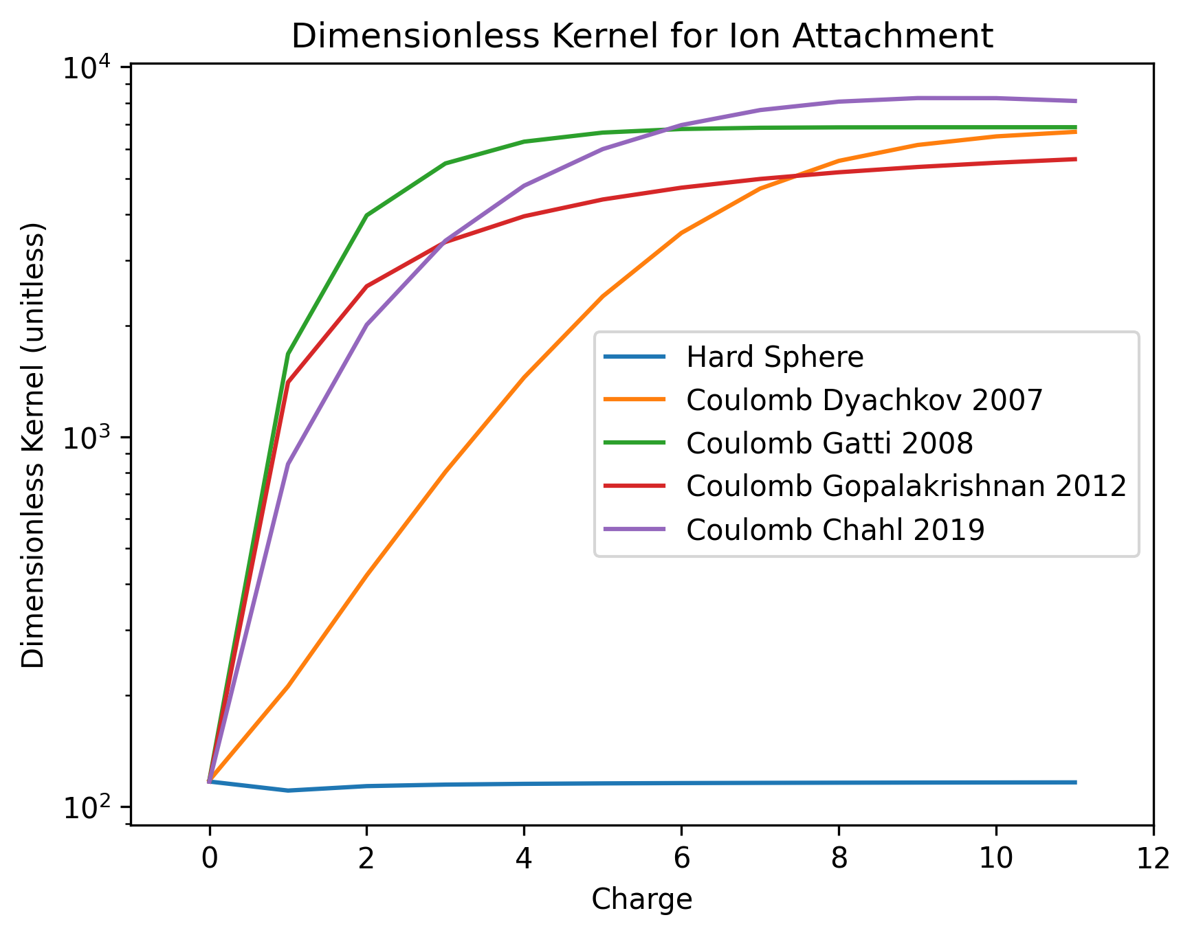
Dimensional Kernel
Section titled “Dimensional Kernel”The code below transforms dimensionless coagulation kernels into dimensional kernels using the get_dimensional_kernel function from the Particula library. This transformation is necessary because dimensionless kernels provide normalized interaction rates that need to be rescaled to physical units for real-world applications.
The function get_dimensional_kernel requires several physical parameters to properly scale the dimensionless kernel:
-
Sum of Particle Radii (
sum_of_radii)sum_of_radii = particle_radius[:, np.newaxis] + particle_radius[np.newaxis, :]- This computes a 2D array where each entry represents the sum of the radii of two interacting particles.
- The broadcasting ensures that each pairwise combination of particle sizes is considered.
-
Reduced Mass (
reduced_mass)- The reduced mass is a standard concept in two-body problems, defined as: μ = {m_1 m_2}/{m_1 + m_2}
- This accounts for how mass differences influence the dynamics of collisions.
-
Reduced Friction Factor (
reduced_friction_factor)reduced_friction_factor = par.util.get_reduced_self_broadcast(friction_factor)- The friction factor relates to the drag experienced by particles in a medium.
- Using a reduced version ensures that the calculation remains valid for all possible particle pairings.
-
Applying Scaling to Compute Dimensional Kernel Each dimensional kernel is computed by combining:
- The precomputed dimensionless kernel
- The coulomb potential ratio, which determines the electrostatic influence.
- The sum of radii, reduced mass, and reduced friction factor, which introduce physical units.
The transition from dimensionless to dimensional kernels is required to:
- Convert relative interaction rates into absolute coagulation frequencies (e.g., collisions per second per cubic meter).
Kernel via System State
Section titled “Kernel via System State”The shortest method to get the kernel is via par.dynamics.get_coulomb_kernel_dyachkov2007_via_system_state. This function combines the steps above into a single call, allowing for a more streamlined approach to obtaining the kernel.
However, depending on you program the properties calculated above may already be available. In this case, you can use the par.dynamics.get_coulomb_kernel_dyachkov2007 function to reduce duplicate calculations.
Python · section 4
sum_of_radii = particle_radius[:, np.newaxis] + particle_radius[np.newaxis, :]reduced_mass = par.util.get_reduced_self_broadcast(particle_mass)reduced_friction_factor = par.util.get_reduced_self_broadcast(friction_factor)
# hard sphere dimensional kernelhard_sphere_dimensional_kernel = par.dynamics.get_dimensional_kernel(    dimensionless_kernel=hard_sphere_dimensionless_kernel,    coulomb_potential_ratio=coulomb_potential_ratio,    sum_of_radii=sum_of_radii,    reduced_mass=reduced_mass,    reduced_friction_factor=reduced_friction_factor,)
# coulomb dimensional kernel for Dyachkov et al. (2007)coulomb_dyachkov2007_dimensional_kernel = par.dynamics.get_dimensional_kernel(    dimensionless_kernel=coulomb_dyachkov2007_dimensionless_kernel,    coulomb_potential_ratio=coulomb_potential_ratio,    sum_of_radii=sum_of_radii,    reduced_mass=reduced_mass,    reduced_friction_factor=reduced_friction_factor,)
# coulomb dimensional kernel for Gatti et al. (2008)coulomb_gatti2008_dimensional_kernel = par.dynamics.get_dimensional_kernel(    dimensionless_kernel=coulomb_gatti2008_dimensionless_kernel,    coulomb_potential_ratio=coulomb_potential_ratio,    sum_of_radii=sum_of_radii,    reduced_mass=reduced_mass,    reduced_friction_factor=reduced_friction_factor,)
# coulomb dimensional kernel for Gopalakrishnan et al. (2012)coulomb_g2012_dimensional_kernel = par.dynamics.get_dimensional_kernel(    dimensionless_kernel=coulomb_g2012_dimensionless_kernel,    coulomb_potential_ratio=coulomb_potential_ratio,    sum_of_radii=sum_of_radii,    reduced_mass=reduced_mass,    reduced_friction_factor=reduced_friction_factor,)
# coulomb dimensional kernel for Chahl et al. (2019) via system statecoulomb_chahl20019_dimensional_kernel = par.dynamics.get_coulomb_kernel_dyachkov2007_via_system_state(    particle_radius=particle_radius,    particle_mass=particle_mass,    particle_charge=charge,    temperature=temperature,    pressure=pressure,)
# plot the first index ion attachment to the other particlesfig, ax = plt.subplots()ax.plot(charge[1:], hard_sphere_dimensional_kernel[0, 1:], label="Hard Sphere")ax.plot(    charge[1:],    coulomb_dyachkov2007_dimensional_kernel[0, 1:],    label="Coulomb Dyachkov 2007",)ax.plot(    charge[1:],    coulomb_gatti2008_dimensional_kernel[0, 1:],    label="Coulomb Gatti 2008",)ax.plot(    charge[1:],    coulomb_g2012_dimensional_kernel[0, 1:],    label="Coulomb Gopalakrishnan 2012",)ax.plot(    charge[1:],    coulomb_chahl20019_dimensional_kernel[0, 1:],    label="Coulomb Chahl 2019",)ax.set_yscale("log")ax.set_xlim(-1, 12)ax.set_xlabel("Charge (integer count)")ax.set_ylabel(r"Dimensional Kernel $m^3/s$")ax.set_title("Dimensional Kernel for Ion Attachment")ax.legend(loc="lower right")plt.show()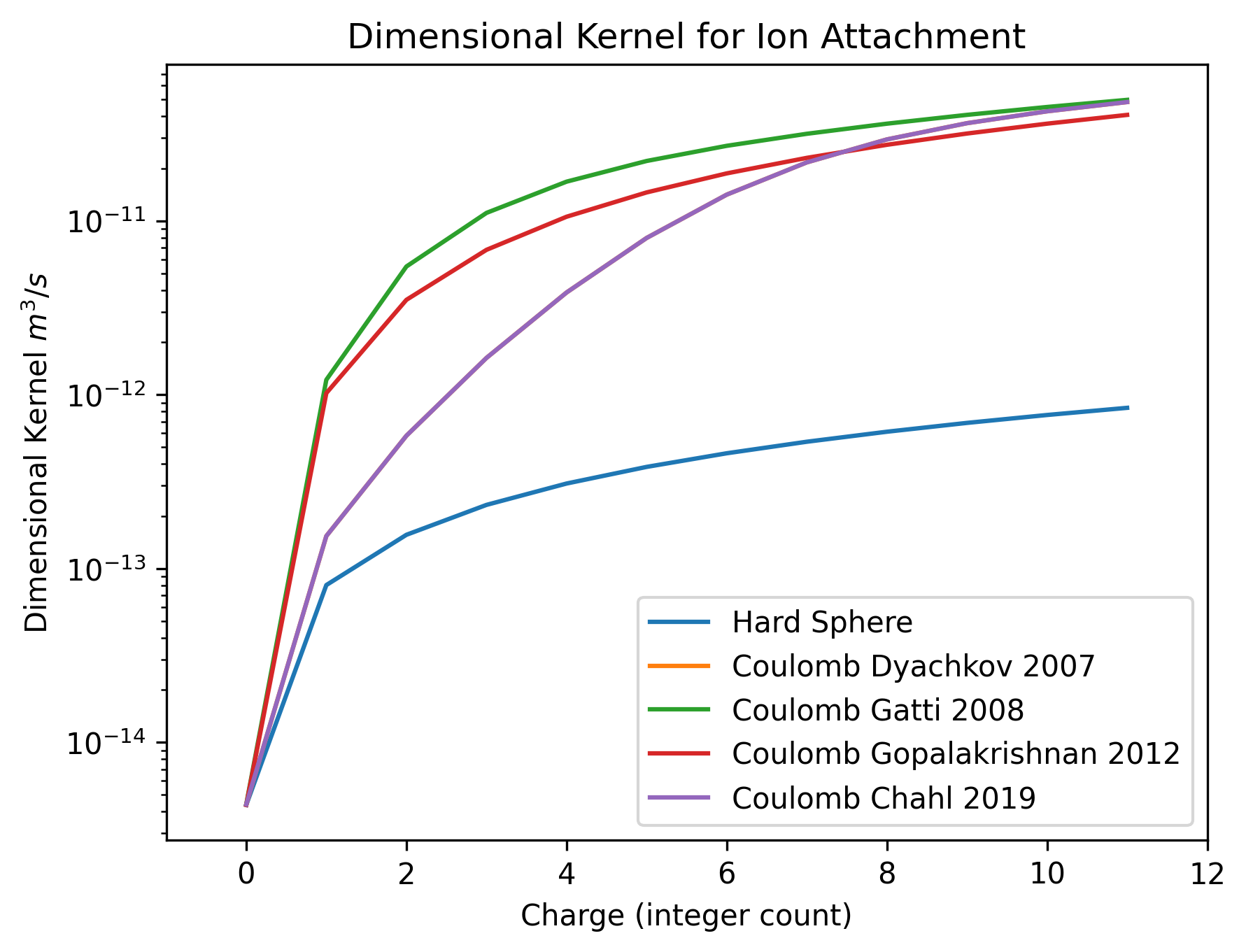
Conclusion
Section titled “Conclusion”In this notebook, we explored the ion-particle coagulation process by calculating various dimensionless and dimensional kernels for different coagulation approximations. The key steps and findings are summarized below:
-
Environmental and Particle Properties Setup:
- Temperature: 278.0 K
- Particle radii ranged from 0.45 nm to 3 nm.
- Charges ranged from -1 to +12.
- Particle densities were set to 1700 kg/m³ and 1860 kg/m³.
-
Key Calculations:
- Mass Calculation: Using the volume of a sphere and given densities.
- Dynamic Viscosity: Obtained using the
par.gas.get_dynamic_viscosity()function. - Knudsen Number: Calculated using the mean free path and particle radius.
- Friction Factor: Influences the motion and diffusion of particles.
- Coulomb Potential Ratio: Determines the effect of electrostatic interactions.
- Diffusive Knudsen Number: Governs diffusion behavior.
-
Dimensionless Kernels:
- Hard-Sphere Kernel: Represents baseline collision frequency with idealized electrostatic interactions.
- Coulomb Kernels: Incorporate electrostatic interactions for different parameterization (Dyachkov 2007, Gatti 2008, Gopalakrishnan 2012, Chahl 2019).
-
Dimensional Kernels:
- Transformed dimensionless kernels into dimensional kernels using physical parameters.
- Plotted the dimensional kernels for ion attachment to other particles.
The analysis provided insights into how different coagulation approximations affect the collision frequencies and coagulation rates of charged particles. The results can be used to better understand and model aerosol dynamics in various environmental and industrial applications.
Explore this topic: Charged particles and ions