

From stored vapor mass to saturation
From stored vapor mass to saturation
Section titled “From stored vapor mass to saturation”Which gas is closest to saturation when the species have different molecular weights and vapor pressures? This CPU example stores water, butanol, and styrene in explicit order, then evaluates pure vapor pressures and saturation ratios. The outcome is a thermodynamic diagnostic, not a condensation time history. Read vapor-pressure conventions before changing coefficients.
Python · section 1
import matplotlib.pyplot as pltimport numpy as npimport particula as parMatch a property model to each species
Section titled “Match a property model to each species”Water uses the Buck relation. The organics use NIST Antoine coefficients,
converted from bar to the implementation’s mmHg-based logarithm and from
T + C to T - c. The vapor-pressure example gives the
source table and conversion. The 304–333 K sweep lies within both selected
organic fits. A common method interface does not make coefficients interchangeable.
Python · section 2
# Define the coefficients for Butanol using the Antoine equation.# 'a', 'b', and 'c' are coefficients specific to the Antoine equation used to calculate vapor pressure.butanol_coefficients = {    "a": 4.54607 + np.log10(1e5 / 133.322387415),    "b": 1351.555,    "c": 93.34,}# Create a vapor pressure strategy for Butanol using the Antoine equation.butanol_antione = par.gas.VaporPressureFactory().get_strategy(    strategy_type="antoine", parameters=butanol_coefficients)
# Define the coefficients for Styrene, similar to Butanol, using the# Antoine equation.styrene_coefficients = {    "a": 4.21948 + np.log10(1e5 / 133.322387415),    "b": 1525.059,    "c": 56.379,}# Create a vapor pressure strategy for Styrene using the Antoine equation.styrene_antione = par.gas.VaporPressureFactory().get_strategy(    strategy_type="antoine", parameters=styrene_coefficients)
# Water uses a different model for vapor pressure calculation called the Buck equation.# The Buck equation is particularly suited for water vapor calculations.# No additional parameters are required to be passed for the Buck equation# in this instance.water_buck = par.gas.VaporPressureFactory().get_strategy(    strategy_type="water_buck")
Construct native gas data
Section titled “Construct native gas data”The water builder converts g/mol and micrograms/m^3 into SI. Concentration has shape (boxes, species); molar mass and flags have one entry per species.
Python · section 3
water_species = ( par.gas.GasDataBuilder() .set_names(["Water"]) .set_molar_mass([18.01528], "g/mol") .set_partitioning([True]) .set_concentration([1e2], "ug/m^3") .build())organic_names = ["butanol", "styrene"]organic_vapor_pressure = [butanol_antione, styrene_antione]organic_species = ( par.gas.GasDataBuilder() .set_names(organic_names) .set_molar_mass([0.074121, 104.15e-3], "kg/mol") .set_partitioning([True, True]) .set_concentration([2e-6, 1e-9], "kg/m^3") .build())print(water_species)print(organic_species)GasData(name=['Water'], molar_mass=array([0.01801528]), concentration=array([[1.e-07]]), partitioning=array([ True]))
GasData(name=['butanol', 'styrene'], molar_mass=array([0.074121, 0.10415 ]), concentration=array([[2.e-06, 1.e-09]]), partitioning=array([ True, True]))Compare pure-substance reference pressures
Section titled “Compare pure-substance reference pressures”Evaluate each strategy in the same order as its gas storage. The first plot compares pure vapor pressure in pascals on a logarithmic axis. It describes each substance’s saturation reference, not the partial pressure of the stored mixture. The curves do not by themselves rank how saturated the gases are: their actual mass concentrations differ.
Python · section 4
temperature_range = np.linspace(304.0, 333.0, 100)organic_pure_vapor_pressure = np.stack(    [        strategy.pure_vapor_pressure(temperature_range)        for strategy in organic_vapor_pressure    ])water_pure_vapor_pressure = water_buck.pure_vapor_pressure(temperature_range)
# Plotting the vapor pressure curves for the organic species.fig, ax = plt.subplots(figsize=(8, 6))for i in range(len(organic_names)):    ax.plot(        temperature_range,        organic_pure_vapor_pressure[i],        label=organic_names[i],    )ax.plot(temperature_range, water_pure_vapor_pressure, label="Water")ax.set_xlabel("Temperature (K)")ax.set_ylabel("Vapor Pressure (Pa)")ax.set_yscale("log")ax.legend()plt.show()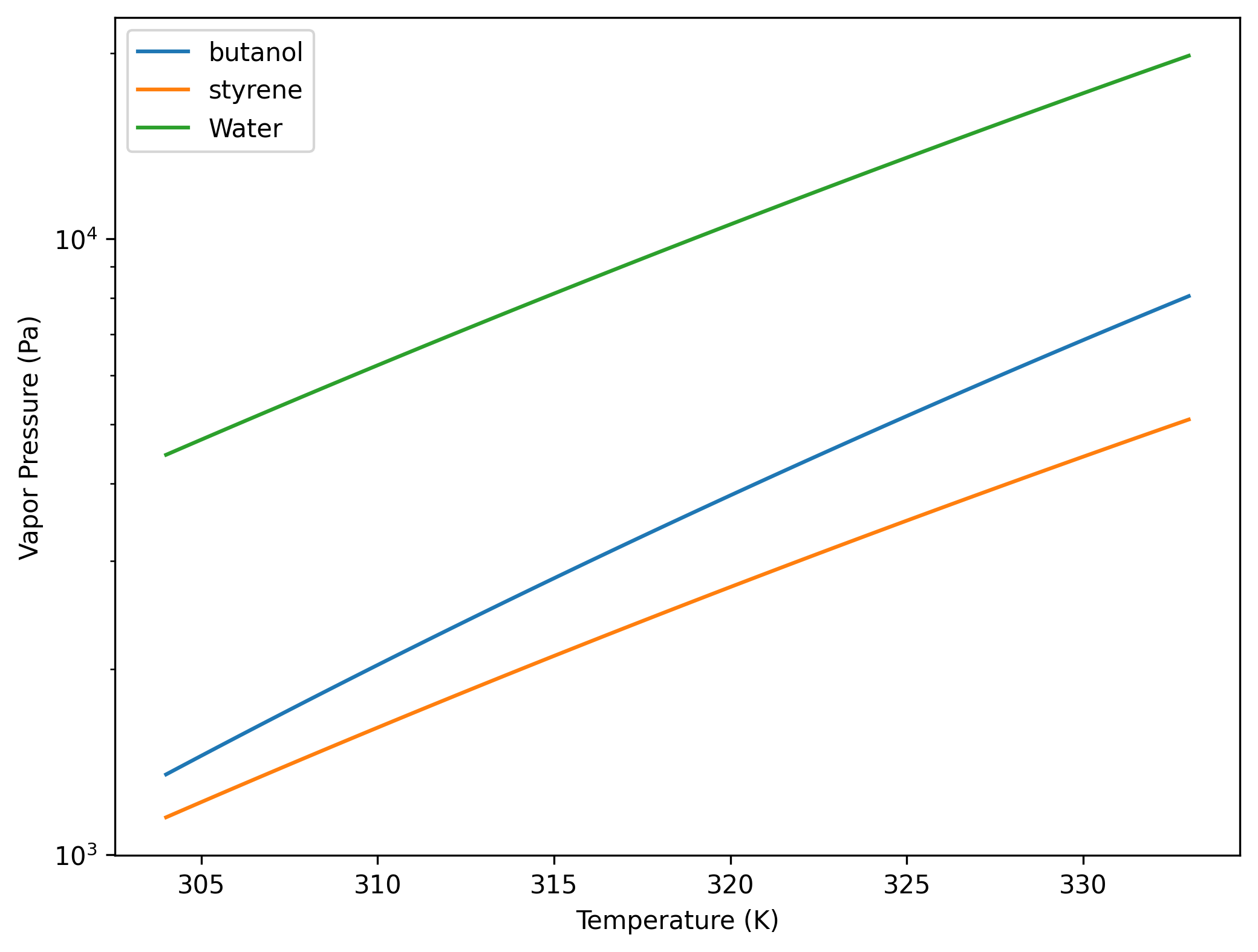
Compare the mixture with those references
Section titled “Compare the mixture with those references”For each fixed gas mass concentration, the ideal-gas conversion gives partial pressure; dividing by pure vapor pressure gives saturation ratio. The second plot uses a logarithmic axis to resolve the small ratios for this dilute mixture. A ratio of one refers to the pure-substance reference. Particle composition and curvature would change the relevant surface equilibrium pressure.
Python · section 5
organic_saturation_ratio = np.stack(    [        strategy.saturation_ratio(            organic_species.concentration[0, lane],            organic_species.molar_mass[lane],            temperature_range,        )        for lane, strategy in enumerate(organic_vapor_pressure)    ])water_saturation_ratio = water_buck.saturation_ratio(    water_species.concentration[0, 0],    water_species.molar_mass[0],    temperature_range,)
# Plotting the saturation ratio curves for the organic species.fig, ax = plt.subplots(figsize=(8, 6))for i in range(len(organic_names)):    ax.plot(        temperature_range, organic_saturation_ratio[i], label=organic_names[i]    )ax.plot(temperature_range, water_saturation_ratio, label="Water")ax.set_yscale("log")ax.set_xlabel("Temperature (K)")ax.set_ylabel("Saturation Ratio")ax.legend()plt.show()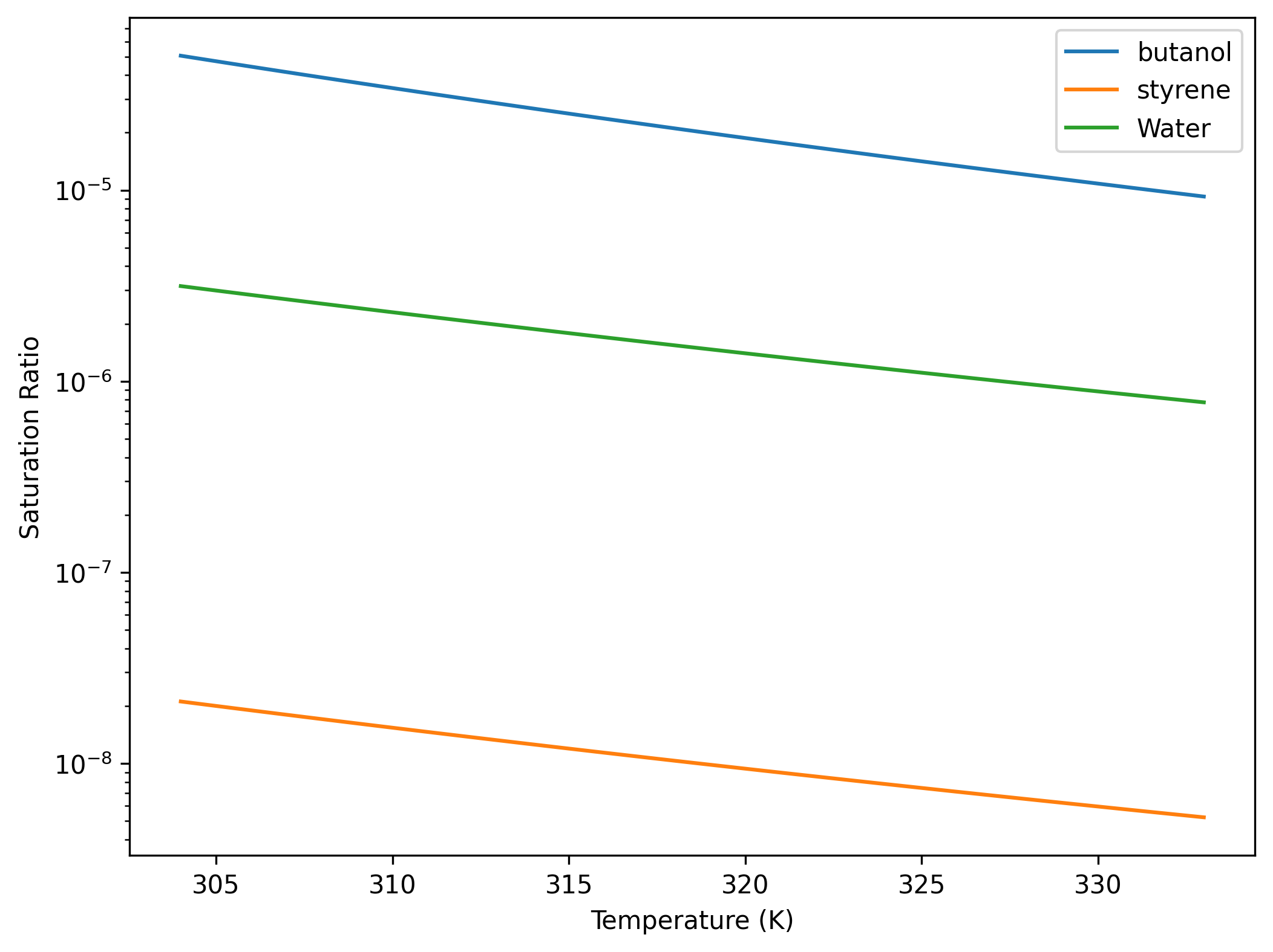
Separate abundance from volatility
Section titled “Separate abundance from volatility”The printed water concentration demonstrates the unit conversion from 100 µg m⁻³ to 10⁻⁷ kg m⁻³. The plots then separate two controls: the chosen vapor-pressure model and the amount of vapor actually present. A larger pure vapor pressure does not automatically imply a larger saturation ratio.
To adapt this to measured vapor concentrations, preserve species order and coefficient provenance, propagate measurement uncertainty, and inspect the ratio over the experimental temperature range. Then add particle activity and curvature before predicting uptake. Continue with the prescribed-environment sweep to isolate cooling effects.
Explore this topic: Gas and environment