

Competition for a finite water-vapor reservoir
Competition for a finite water-vapor reservoir
Section titled “Competition for a finite water-vapor reservoir”What changes when particles consume the vapor that drives their growth? This CPU calculation follows individual component masses while updating a shared gas reservoir. It contrasts with the maintained-vapor assumption in the moving-bin example, but uses different initial conditions rather than forming a direct numerical comparison.
The goal is to read size-distribution evolution together with water depletion and particle mass. Familiarity with represented counts and volume and κ activity helps interpret the bookkeeping.
Python · section 1
# In Colab uncomment the following command to install particula:# Install from the repository root: `python -m pip install -e ".[extra]"`import matplotlib.pyplot as pltimport numpy as npimport particula as parfrom particula.dynamics.condensation.species_mapping import ( CondensationSpeciesMap,)Specify a closed material inventory
Section titled “Specify a closed material inventory”The initial water saturation ratio is 1.025 at 298.15 K. Gas updates are enabled, so this is an initial condition, not humidity maintained throughout the run. Temperature remains fixed; latent-heat feedback is absent. Water and a low-volatility hygroscopic component share the particle state.
The legacy gas label NH4HSO4 is an identifier, not a complete chemical model.
The supplied molar mass, density, κ, and surface tension require a consistent
material specification before applying this setup to a particular salt.
Python · section 2
initial_water_vapor_activity = 1.025  # Relative humidity/100
# Ammonium sulfate and water vapor pressuremolar_mass_ammonium_sulfate = 132.14e-3  # kg/molmolar_mass_water = 18.015e-3  # kg/molparameters_vapor = {    "vapor_pressure": 1e-24,    "vapor_pressure_units": "Pa",}vapor_pressure_ammonium = par.gas.VaporPressureFactory().get_strategy(    "constant", parameters_vapor)vapor_pressure_water = par.gas.VaporPressureFactory().get_strategy("water_buck")
water_sat = vapor_pressure_water.saturation_concentration(    molar_mass=molar_mass_water, temperature=298.15)water_concentration = water_sat * initial_water_vapor_activity
gas_phase = (    par.gas.GasDataBuilder()    .set_molar_mass(        np.array([molar_mass_water, molar_mass_ammonium_sulfate]), "kg/mol"    )    .set_concentration(np.array([water_concentration, 1e-30]), "kg/m^3")    .set_names(["H2O", "NH4HSO4"])    .set_partitioning([True, True])    .build())
environment = par.gas.EnvironmentData(    temperature=[298.15],    pressure=[101325.0],    saturation_ratio=[[water_concentration / water_sat, 0.0]],)
Resolve the distribution without confusing radius and diameter
Section titled “Resolve the distribution without confusing radius and diameter”The samples are used as radii in the spherical mass calculation. The two radius scales are 100 and 400 nm, and 10,000 unit-count particles occupy 1 cm³. Thus the initial number density is 10¹⁰ m⁻³. The fixed seed selects one initial sample; it does not quantify uncertainty in a measured population.
Each slot initially has dry-component mass and zero water. As water accumulates, its activity and the curvature correction change, allowing size-dependent responses even though all particles share one vapor reservoir.
Python · section 3
density = 1.77e3  # kg/m^3volume_sim = 1 * par.util.get_unit_conversion("cm^3", "m^3")  # m^3number_of_samples = 10_000
np.random.seed(42)
# Generate a particle distribution using a lognormal sample distribution# This distribution has a mean particle diameter (mode) and geometric standard deviation (GSD)particle_sample = par.particles.get_lognormal_sample_distribution(    mode=np.array([100, 400]) * 1e-9,    geometric_standard_deviation=np.array([1.3, 1.4]),    number_of_particles=np.array([1, 0.5]),  # relative to each mode    number_of_samples=number_of_samples,  # Number of samples for particle distribution)
# Calculate the mass of each particle in the sample, assuming density of 1500 kg/m^3particle_mass = (    4 / 3 * np.pi * particle_sample**3 * density)  # Particle mass in kg
mass_speciation = np.column_stack(    [particle_mass * 0, particle_mass])  # water, ammonium sulfatedensities = np.array([1000, density])  # kg/m^3
# kappa activityactivity_strat = (    par.particles.ActivityKappaParameterBuilder()    .set_density(densities, "kg/m^3")    .set_kappa(np.array([0.0, 0.61]))    .set_molar_mass(        np.array([molar_mass_water, molar_mass_ammonium_sulfate]), "kg/mol"    )    .set_water_index(0)    .build())
surface_strat = (    par.particles.SurfaceStrategyVolumeBuilder()    .set_density(densities, "kg/m^3")    .set_surface_tension(np.array([0.072, 0.092]), "N/m")    .build())

# Build a resolved mass representation for each particle# This defines how particle mass, activity, and surface are representedresolved_masses = par.particles.create_resolved_particle_data(    masses=mass_speciation,    density=densities,    volume=volume_sim,)aerosol_resolved = par.Aerosol(    particles=resolved_masses,    gas=gas_phase,    environment=environment,)
print(aerosol_resolved)
ParticleData(masses=array([[[0.00000000e+00, 1.09610890e-17],
[0.00000000e+00, 1.23441527e-17],
[0.00000000e+00, 6.16625122e-18],
...,
[0.00000000e+00, 2.51160058e-16],
[0.00000000e+00, 3.08530181e-17],
[0.00000000e+00, 1.86701325e-16]]], shape=(1, 10000, 2)), concentration=array([[1., 1., 1., ..., 1., 1., 1.]], shape=(1, 10000)), charge=array([[0., 0., 0., ..., 0., 0., 0.]], shape=(1, 10000)), density=array([1000., 1770.]), volume=array([1.e-06]), distribution_type='particle_resolved', radius_grid=None)
GasData(name=['H2O', 'NH4HSO4'], molar_mass=array([0.018015, 0.13214 ]), concentration=array([[2.360191e-02, 1.000000e-30]]), partitioning=array([ True, True]))
EnvironmentData(temperature=array([298.15]), pressure=array([101325.]), saturation_ratio=array([[1.025, 0. ]]))Couple particle uptake to gas depletion
Section titled “Couple particle uptake to gas depletion”update_gases=True couples material transfer to the gas inventory. The loop
records the initial state and then 999 advances of 0.01 s, each with ten
substeps; the last recorded time is 9.99 s. At every recorded state, the
assertion checks each gas-plus-particle material inventory using physical volume.
The diagnostic water saturation ratio is recomputed from current gas and temperature. The environment’s stored initial ratio is not the evolving humidity record. Conservation checks constrain material accounting, while timestep refinement would test trajectory accuracy.
Python · section 4
# define the condensation processcondensation_isothermal = par.dynamics.CondensationIsothermal(    activity_strategy=activity_strat,    surface_strategy=surface_strat,    vapor_pressure_strategy=[vapor_pressure_water, vapor_pressure_ammonium],    species_map=CondensationSpeciesMap(("H2O", "NH4HSO4"), ((0, 0), (1, 1))),    molar_mass=np.array(        [molar_mass_water, molar_mass_ammonium_sulfate]    ),  # kg/mol    diffusion_coefficient=2e-5,  # m^2/s    accommodation_coefficient=1,  # makes things go slower/faster    update_gases=True,)condensation_process = par.dynamics.MassCondensation(    condensation_strategy=condensation_isothermal)
# Set up time and sub-steps for the coagulation processtotal_time = 10time_step = 0.01sub_steps = 10
# binsbins_lognormal = np.logspace(-8, -4, 200)

# output arraystime = np.arange(0, total_time, time_step)total_mass_resolved = np.ones_like(time, dtype=np.float64)number_distribution_resolved = np.zeros((len(time), number_of_samples))number_distribution_binned = np.zeros((len(time), len(bins_lognormal) - 1))total_number_resolved = np.ones_like(time, dtype=np.float64)water_saturation_in_time = np.ones_like(time, dtype=np.float64)
print(f"Total iterations to do: {len(time) * sub_steps}")
Total iterations to do: 10000Python · section 5
# Independent per-species extensive inventory before the full published run.initial_inventory = (    np.sum(        resolved_masses.masses * resolved_masses.concentration[..., None],        axis=1,    )    + gas_phase.concentration * resolved_masses.volume[:, None])# Simulation loopfor i, _t in enumerate(time):    if i > 0:        # Perform condensation for the resolved aerosol        aerosol_resolved = condensation_process.execute(            aerosol_resolved, time_step, sub_steps        )
    current_inventory = (        np.sum(            resolved_masses.masses * resolved_masses.concentration[..., None],            axis=1,        )        + gas_phase.concentration * resolved_masses.volume[:, None]    )    np.testing.assert_allclose(        current_inventory, initial_inventory, rtol=1e-12, atol=1e-30    )    if not np.all(np.isfinite(resolved_masses.masses)) or np.any(        resolved_masses.masses < 0    ):        raise AssertionError("Nonphysical particle masses")    total_mass_resolved[i] = (        aerosol_resolved.particles.species_mass_density.sum()    )    number_distribution_resolved[i, :] = aerosol_resolved.particles.radii[0]    number_distribution_binned[i, :], edges = np.histogram(        number_distribution_resolved[i, :], bins=bins_lognormal    )    total_number_resolved[i] = np.sum(number_distribution_resolved[i, :] > 0)    water_saturation_in_time[i] = vapor_pressure_water.saturation_ratio(        aerosol_resolved.gas.concentration[0, 0],        molar_mass_water,        aerosol_resolved.environment.temperature[0],    )

number_distribution_binned = number_distribution_binned / volume_sim
print(aerosol_resolved)
ParticleData(masses=array([[[1.46138086e-15, 1.09610890e-17],
[1.69264383e-15, 1.23441527e-17],
[7.10570981e-16, 6.16625122e-18],
...,
[6.78233789e-14, 2.51160058e-16],
[5.14965328e-15, 3.08530181e-17],
[4.88385892e-14, 1.86701325e-16]]], shape=(1, 10000, 2)), concentration=array([[1., 1., 1., ..., 1., 1., 1.]], shape=(1, 10000)), charge=array([[0., 0., 0., ..., 0., 0., 0.]], shape=(1, 10000)), density=array([1000., 1770.]), volume=array([1.e-06]), distribution_type='particle_resolved', radius_grid=None)
GasData(name=['H2O', 'NH4HSO4'], molar_mass=array([0.018015, 0.13214 ]), concentration=array([[2.30009156e-02, 1.00000000e-30]]), partitioning=array([ True, True]))
EnvironmentData(temperature=array([298.15]), pressure=array([101325.]), saturation_ratio=array([[1.025, 0. ]]))Read size, mass, and vapor together
Section titled “Read size, mass, and vapor together”The first plot compares the initial distribution, the selected 1 s snapshot, and the last recorded state. The legend’s “CCN overshoot” label identifies that chosen snapshot; it is not an independently detected activation threshold. Histogram values are number per volume in each interval, not density per metre.
The time–radius map shows how occupancy shifts between intervals; empty bins are omitted from the logarithmic color scale. The final panel relates particle mass density to the recomputed water saturation ratio. Size changes alone cannot show whether the vapor reservoir was depleted.
Python · section 6
# plot the initial and final distributionsfig, ax = plt.subplots(figsize=(8, 5))
ax.bar(    edges[:-1],    number_distribution_binned[0, :],    width=np.diff(edges),    align="edge",    label="Resolved initial",    color="red",    alpha=0.7,)plot_index = 100ax.bar(    edges[:-1],    number_distribution_binned[plot_index, :],    width=np.diff(edges),    align="edge",    label="CCN overshoot time: {:.1f} s".format(time[plot_index]),    color="purple",    alpha=0.5,)ax.bar(    edges[:-1],    number_distribution_binned[-1, :],    width=np.diff(edges),    align="edge",    label="Resolved final",    color="blue",    alpha=0.7,)ax.set_yscale("log")ax.set_xscale("log")ax.set_xlabel("Particle radius (m)")ax.set_ylabel("Number concentration (m^-3)")ax.legend()plt.show()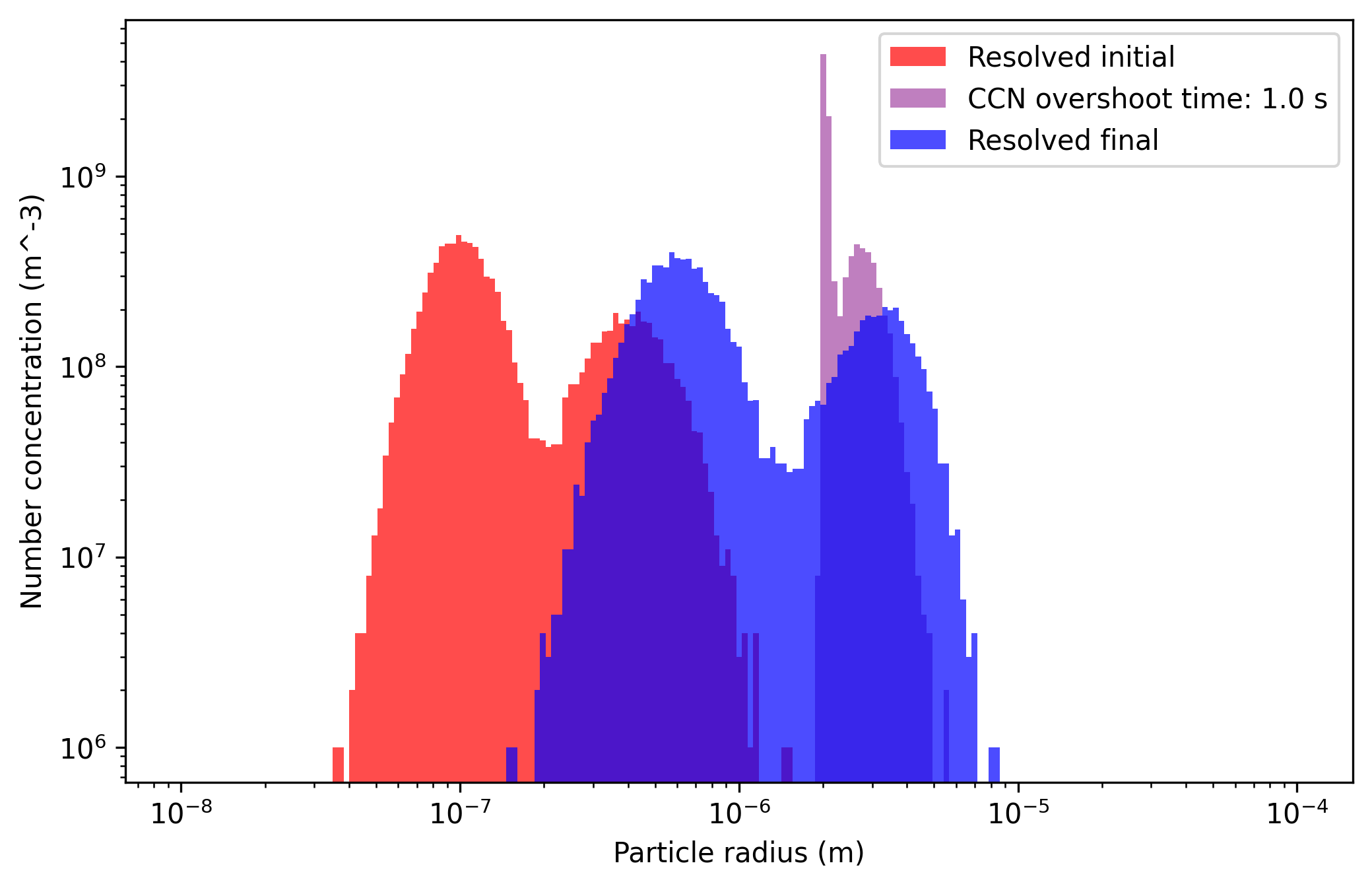
Python · section 7
fig, ax = plt.subplots(figsize=(8, 5))
# Swap X and Y to reverse axesX, Y = np.meshgrid(    time, edges[:-1])  # Now time is on the x-axis and edges on the y-axis
# Plot the contour with updated X and Ylog_of_number_distribution_binned = np.log10(    number_distribution_binned,    out=np.nan * np.ones_like(number_distribution_binned),    where=number_distribution_binned > 0,)contour = ax.contourf(    X,    Y,    log_of_number_distribution_binned.T,    cmap="viridis",    vmin=5,)
# Add the color barcbar = fig.colorbar(contour)cbar.set_label("Log10 of Number concentration (m^-3)")
ax.set_ylim([1e-8, 1e-5])  # Set limits for y-axis
# Set axis labelsax.set_yscale("log")  # Log scale for particle radius on y-axisax.set_xlabel("Time (s)")ax.set_ylabel("Particle radius (m)")fig.tight_layout()plt.show()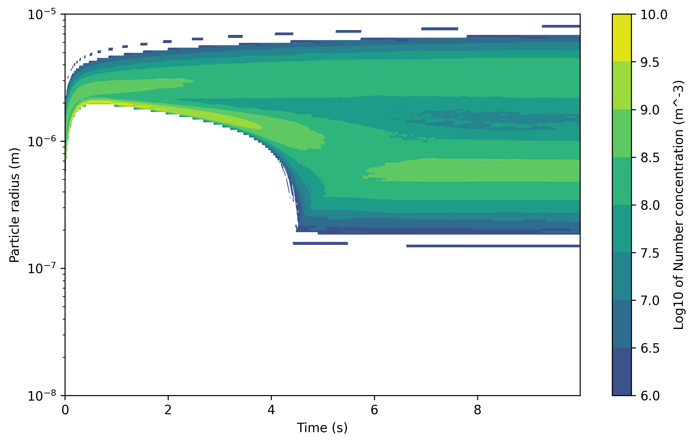
Python · section 8
# plot the total mass and water saturation on twin y-axisfig, ax1 = plt.subplots(figsize=(8, 5))
ax1.plot(time, total_mass_resolved, label="Total mass", color="blue")ax1.set_xlabel("Time (s)")ax1.set_ylabel("Total Particle mass (kg/m^3)", color="blue")ax1.tick_params(axis="y", labelcolor="blue")
ax2 = ax1.twinx()ax2.plot(time, water_saturation_in_time, label="Water saturation", color="red")ax2.set_ylabel("Water saturation", color="red")ax2.tick_params(axis="y", labelcolor="red")
fig.tight_layout()plt.show()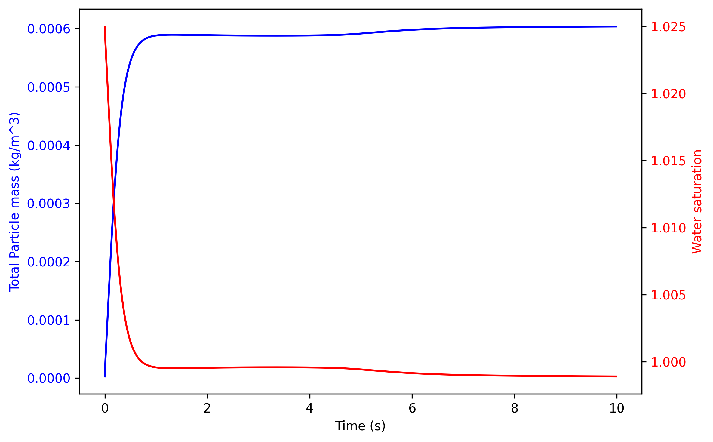
What the coupled history establishes
Section titled “What the coupled history establishes”The saved run gains particle water while the gas water concentration decreases; per-material assertions keep their combined inventory fixed. These diagnostics establish transfer within the specified closed, isothermal system. A size histogram alone cannot establish which individual particles activated or whether a transient is numerically resolved.
For a cloud-activation question, define an explicit activation diagnostic and track individual radius histories alongside the vapor budget. Repeat the initial sampling and halve the timestep before interpreting a transient peak. To study feedback from heating, add a thermal model rather than interpreting the isothermal trajectory as adiabatic. The latent-heat bookkeeping example shows the energy signal that such a model would need.
Explore this topic: Population growth and vapor reservoirs