

Turn measurements into particle state
Turn measurements into particle state
Section titled “Turn measurements into particle state”A size spectrum, a table of component masses, and a fitted lognormal population are different starting points for the same model. This CPU example constructs all three and asks: which quantities describe individual particles, and which describe how many particles they represent?
You will be able to choose an initializer, supply units, and interpret the
resulting histograms. Read size distributions for
bin number versus density. ParticleData stores masses, weights, charge,
densities, and volume; activity and surface models remain separate configuration.
Python · section 1
import matplotlib.pyplot as pltimport numpy as npimport particula as parInitialize from radii with explicit units
Section titled “Initialize from radii with explicit units”Discrete concentrations are number densities. Binned data uses a unit reference volume; per-particle masses follow the spherical volume formula.
Python · section 2
input_radius_nm = np.array([100, 200, 300], dtype=np.float64)input_concentration_cm3 = np.array([1e2, 1e3, 1e4], dtype=np.float64)particle_data = par.particles.create_particle_data_from_radii( radii=input_radius_nm, radius_units="nm", concentration=input_concentration_cm3, concentration_units="1/cm^3", density=2.5, density_units="g/cm^3", distribution_type="discrete",)surface_strategy = ( par.particles.SurfaceStrategyMassBuilder() .set_surface_tension(0.072, "N/m") .set_density(2.5, "g/cm^3") .build())activity_strategy = par.particles.ActivityFactory().get_strategy("mass_ideal")print("Per-particle mass [kg]:", particle_data.total_mass)print("Radius [m]:", particle_data.radii)print("Material mass density [kg/m^3]:", particle_data.species_mass_density)Per-particle mass [kg]: [[1.04719755e-17 8.37758041e-17 2.82743339e-16]]
Radius [m]: [[1.e-07 2.e-07 3.e-07]]
Material mass density [kg/m^3]: [[2.91225639e-06]]Keep component mass separate from population abundance
Section titled “Keep component mass separate from population abundance”The second initialization gives each of 500 computational bins three material masses and an independently sampled number concentration. The seed fixes this illustration, not a physical composition law. Picograms are converted explicitly to kilograms (1 pg = 10⁻¹⁵ kg), and all material densities are 2,500 kg m⁻³. The printed species mass densities combine per-particle masses with bin weights.
Python · section 3
rng = np.random.default_rng(42)mass_distribution_pg = rng.random((500, 3))concentration_cm3 = rng.random(500) * 1e3speciated_data = ( par.particles.ParticleDataBuilder() .set_distribution_type("discrete") .set_masses(mass_distribution_pg * 1e-15) .set_density(np.full(3, 2500.0)) .set_concentration(concentration_cm3, "1/cm^3") .set_charge(np.zeros(500)) .set_volume(np.array([1.0])) .build())print("Material mass density [kg/m^3]:", speciated_data.species_mass_density)radius = speciated_data.radii[0]masses = speciated_data.total_mass[0]concentration = speciated_data.slot_concentration_density[0]Material mass density [kg/m^3]: [[0.0001296 0.00012898 0.00013249]]Ask what each histogram counts
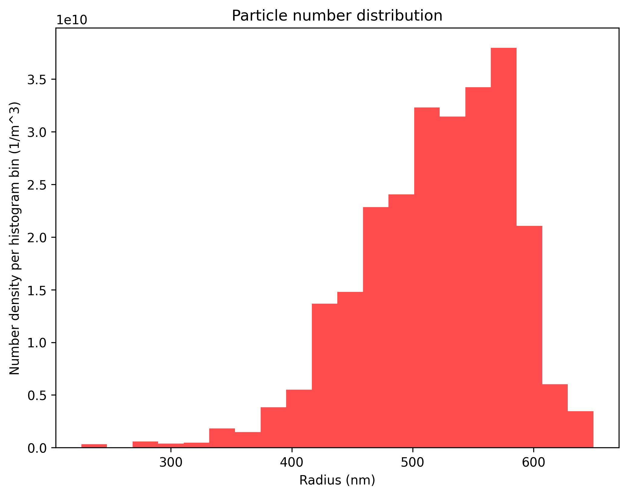
Section titled “Ask what each histogram counts”The first histogram counts computational bins by their per-particle mass. The second weights radii by number concentration and therefore describes physical number per histogram interval in m⁻³. A heavily populated bin can contribute little to the first plot and dominate the second. Compare the ordinates before comparing the shapes; neither plot is a time evolution.
Python · section 4
fig, ax = plt.subplots(figsize=(8, 6))ax.hist(masses * 1e15, bins=20, color="blue", alpha=0.7)ax.set_xlabel("Per-particle mass (pg)")ax.set_ylabel("Computational bins")ax.set_title("Speciated particle masses")plt.show()
fig, ax = plt.subplots(figsize=(8, 6))ax.hist(radius * 1e9, weights=concentration, bins=20, color="red", alpha=0.7)ax.set_ylabel("Number density per histogram bin (1/m^3)")ax.set_xlabel("Radius (nm)")ax.set_title("Particle number distribution")plt.show()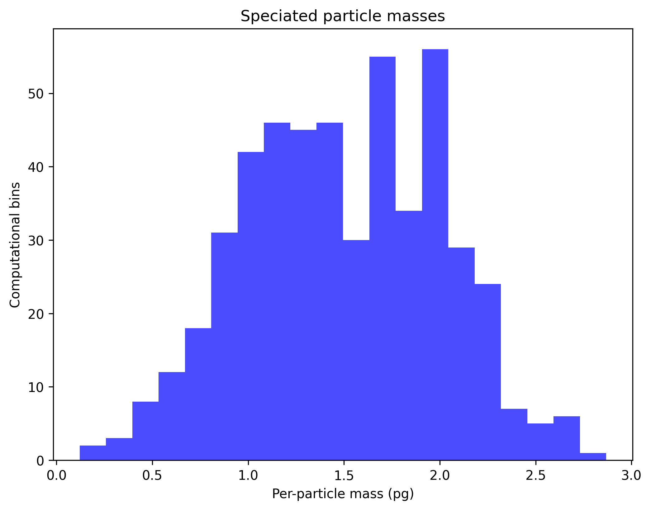
Use a compact population model
Section titled “Use a compact population model”The lognormal preset uses radius scale parameters of 100 nm and 2,000 nm, with 10⁴ cm⁻³ assigned to each component. These are geometric mean radii in the helper’s parameterization, not necessarily the peaks of the plotted bin values. The discrete preset normalizes sampled bin weights to the specified numbers. The plotted ordinate is number per bin, so its total is a sum.
Python · section 5
lognormal_data = par.particles.create_lognormal_binned_particle_data( distribution_type="discrete", mode=[100e-9, 2000e-9], geometric_standard_deviation=[1.5, 2.0], number_concentration=[1e10, 1e10],)fig, ax = plt.subplots(figsize=(8, 6))ax.semilogx( lognormal_data.radii[0], lognormal_data.slot_concentration_density[0], label="Number distribution", color="blue",)ax.set_xlabel("Radius (m)")ax.set_ylabel("Bin number density (1/m^3)")ax.set_title("Lognormal particle population")ax.legend()plt.show()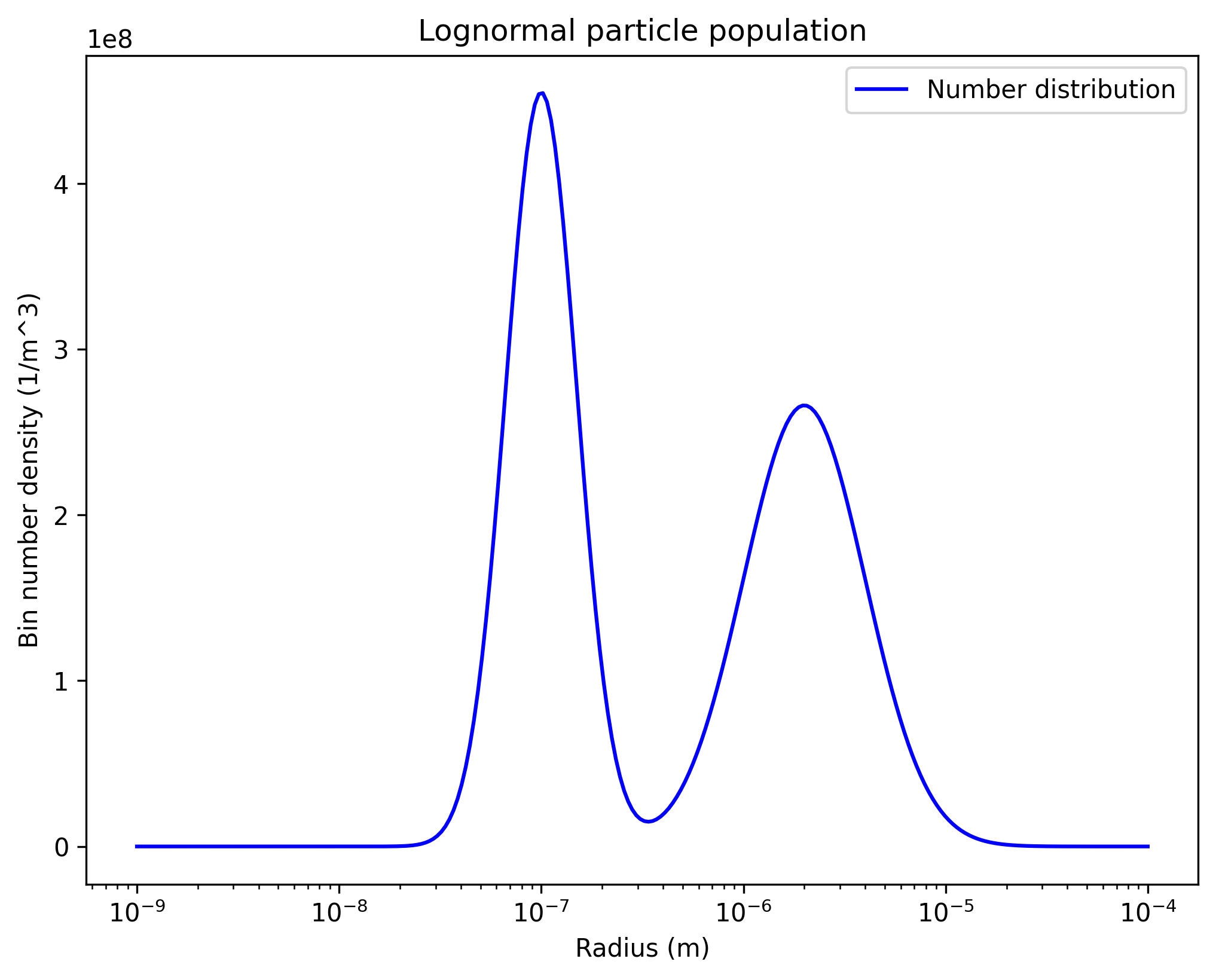
Choose the input that matches the evidence
Section titled “Choose the input that matches the evidence”Radius initialization is appropriate when size and density are known; component mass input retains composition; a lognormal preset expresses a distributional assumption. The two histograms demonstrate why computational sampling and physical abundance must be distinguished. Random input arrays are not measured aerosol composition.
For an instrument-derived population, convert diameter to radius and the reported distribution measure before construction. Compare number and material mass densities with independent integrals of the input, and test sensitivity to binning. If composition varies with size, preserve that information in material lanes rather than replacing it with an effective density without checking its consequences. Continue with native storage.
Explore this topic: Constructing aerosol state