

A compact PDF coagulation calculation
A compact PDF coagulation calculation
Section titled “A compact PDF coagulation calculation”How do you connect a stored size distribution to a physical collision process? This small example isolates the construction and execution choices for Brownian coagulation. Its 200 s horizon is intended to make the workflow easy to inspect; a subtle before/after difference is not evidence that coagulation is absent.
Read distribution measures to connect these concentrations with measurements. The companion alternative representation uses different initial parameters, so the two pages are not a controlled solver comparison.
Python · section 1
# In Colab uncomment the following command to install particula:# Install from the repository root: `python -m pip install -e ".[extra]"`import matplotlib.pyplot as pltimport numpy as npimport particula as parAssign physical meaning to the array
Section titled “Assign physical meaning to the array”The 140 radius nodes span 10 nm–1 µm. The lognormal radius scale is 120 nm, geometric standard deviation 1.5, and target number density 8×10⁸ m⁻³. Concentration stores number per volume per metre of radius (m⁻⁴); integrate over radius to obtain the total. Density is 1000 kg m⁻³.
The environment stays at 298.15 K and 101325 Pa. A zero-concentration carrier fills the gas species axis but is not consumed. Condensation, charging, sources, and external losses are absent.
Python · section 2
# Radius bins (log-spaced)radius_bins = np.logspace(-8, -6, 140)  # m
# Lognormal PDF (concentration per unit size)concentration_pdf = par.particles.get_lognormal_pdf_distribution(    x_values=radius_bins,    mode=np.array([120e-9]),    geometric_standard_deviation=np.array([1.5]),    number_of_particles=np.array([8e8]),  # m^-3 total when integrated)
# Native ambient environment. GasData requires a species axis, so a# zero-concentration, non-partitioning carrier fills that axis. Coagulation# does not consume it; ambient pressure is specified independently.environment = par.gas.EnvironmentData(    temperature=np.array([298.15]),    pressure=np.array([101325.0]),    saturation_ratio=np.zeros((1, 1)),)gas = par.gas.GasData(    name=["carrier"],    molar_mass=np.array([0.02897]),    partitioning=np.array([False]),    concentration=np.zeros((1, 1)),)
# PDF particle representationparticles_pdf = par.particles.create_particle_data_from_radii(    radii=radius_bins,    concentration=concentration_pdf,    distribution_type="continuous_pdf",    density=1000.0,)
aerosol_pdf = par.Aerosol(    particles=particles_pdf, gas=gas.copy(), environment=environment.copy())
Select a strategy consistent with the measure
Section titled “Select a strategy consistent with the measure”The builder specifies Brownian collision physics and the distribution type. The wrapper then advances the aerosol. This separation matters when replacing the collision mechanism: changing a strategy must not silently reinterpret the stored concentration units.
Python · section 3
coagulation_strategy = (    par.dynamics.BrownianCoagulationBuilder()    .set_distribution_type("continuous_pdf")    .build())coagulation_process = par.dynamics.Coagulation(    coagulation_strategy=coagulation_strategy)
print(coagulation_process)
<particula.dynamics.particle_process.Coagulation object at 0x7ff1463f2f30>Preserve a reference before advancing
Section titled “Preserve a reference before advancing”The process mutates the supplied aerosol over 200 s with ten substeps. Copying the initial array preserves the control for the plot. This single timestep choice illustrates execution; the page does not test time-discretization error.
Python · section 4
time_step = 200  # secondssub_steps = 10
pdf_before = aerosol_pdf.particles.concentration[0].copy()radii = aerosol_pdf.particles.radii[0].copy()
aerosol_pdf_after = coagulation_process.execute(    aerosol_pdf, time_step=time_step, sub_steps=sub_steps)pdf_after = aerosol_pdf_after.particles.concentration[0].copy()
Read a small change in the correct units
Section titled “Read a small change in the correct units”The overlay compares number per volume per metre of radius (m⁻⁴). Nearly overlapping curves can hide small changes in total number or mass; peak height alone is not either quantity. For an abundance diagnostic, integrate over radius. To assess material, weight by single-particle mass before applying the same operation.
Python · section 5
fig, ax = plt.subplots(figsize=(8, 5))ax.plot(radii, pdf_before, label="Before", color="tab:blue")ax.plot(radii, pdf_after, label="After", color="tab:orange")ax.set_xscale("log")ax.set_xlabel("Particle radius (m)")ax.set_ylabel(r"PDF concentration ($m^{-4}$)")ax.set_title("PDF coagulation (Brownian, continuous)")ax.legend()ax.grid(alpha=0.3)plt.show()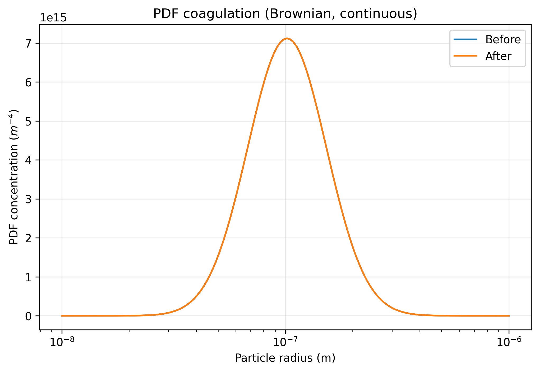
Make the next comparison controlled
Section titled “Make the next comparison controlled”This example supplies a runnable collision calculation and a visual comparison, not a convergence result. The compact PMF/PDF comparison holds initial physical inputs fixed and converts measures before plotting.
For a research adaptation, vary initial abundance while keeping the size law fixed and measure fractional number loss at 200 s. Add mass-drift diagnostics and refine substeps to separate physical concentration sensitivity from numerical error.
The native container retains the generated distribution. Finite-grid coagulation can introduce material drift, and the displayed overlay alone neither measures that drift nor establishes exact conservation.
Explore this topic: Binned populations