

Dns Radial Distribution Comparison
Radial Distribution Function Comparison
Section titled “Radial Distribution Function Comparison”This script compares the radial distribution function g₁₂ between DNS data
and the model predictions from Ayala et al. (2008) for a range of particle radii.
It uses the function get_g12_radial_distribution_ao2008 from the particula
library to compute g₁₂ values over a range of particle radii.
The script then plots these computed values against the DNS datasets
for visual comparison.
Reference: Figure 16 in Ayala et al. (2008).
Ayala, O., Rosa, B., & Wang, L. P. (2008). Effects of turbulence on the geometric collision rate of sedimenting droplets. Part 2. Theory and parameterization. New Journal of Physics, 10. https://doi.org/10.1088/1367-2630/10/7/07501
Usage:
- Run this script to generate and display the comparison graph.
Python · section 1
import numpy as npimport matplotlib.pyplot as pltimport particula as parfrom particula.dynamics.coagulation.turbulent_dns_kernel.g12_radial_distribution_ao2008 import (    get_g12_radial_distribution_ao2008,)

def g12_calc(particle_radius, turbulent_dissipation, reynolds_lambda):    # Define constants and parameters    temperature = 300  # Temperature in Kelvin    particle_density = 1000  # Particle density in kg/m³    fluid_density = 1.0  # Fluid (air) density in kg/m³
    # Basic fluid par.particles    dynamic_viscosity = par.gas.get_dynamic_viscosity(temperature)    kinematic_viscosity = par.gas.get_kinematic_viscosity(        dynamic_viscosity=dynamic_viscosity, fluid_density=fluid_density    )
    # Particle inertia and settling velocity    particle_inertia_time = par.particles.get_particle_inertia_time(        particle_radius=particle_radius,        particle_density=particle_density,        fluid_density=fluid_density,        kinematic_viscosity=kinematic_viscosity,    )
    # Kolmogorov parameters    kolmogorov_time = par.gas.get_kolmogorov_time(        kinematic_viscosity=kinematic_viscosity,        turbulent_dissipation=turbulent_dissipation,    )    kolmogorov_length_scale = par.gas.get_kolmogorov_length(        kinematic_viscosity=kinematic_viscosity,        turbulent_dissipation=turbulent_dissipation,    )    normalized_accel_variance = (        par.gas.get_normalized_accel_variance_ao2008(            re_lambda=reynolds_lambda        )    )    kolmogorov_velocity = par.gas.get_kolmogorov_velocity(        kinematic_viscosity=kinematic_viscosity,        turbulent_dissipation=turbulent_dissipation,    )
    stokes_number = par.particles.get_stokes_number(        particle_inertia_time=particle_inertia_time,        kolmogorov_time=kolmogorov_time,    )
    # Compute g₁₂ Values    g12_values = get_g12_radial_distribution_ao2008(        particle_radius,        stokes_number,        kolmogorov_length_scale,        reynolds_lambda,        normalized_accel_variance,        kolmogorov_velocity,        kolmogorov_time,    )
    return g12_values
DNS Datasets
Section titled “DNS Datasets”We have the following DNS datasets for the radial distribution function g₁₂:
- Case 1: R_λ = 23, ε = 100 cm²/s³
- Case 2: R_λ = 23, ε = 400 cm²/s³
- Case 3: R_λ = 72.4, ε = 100 cm²/s³
- Case 4: R_λ = 72.4, ε = 400 cm²/s³
DNS datasets for radial distribution function are from Ayala et al. (2008).
Python · section 2
# Case R_lambda = 23, turbulent_dissipation = 100 cm2/s3r23_e100 = np.array(    [        [9.937578027, 1.532846715],        [19.98751561, 1.094890511],        [29.91260924, 2.299270073],        [40.02496879, 3.686131387],        [49.95006242, 2.919708029],        [60, 2.737226277],    ])

# case: R_lambda = 23, turbulent_dissipation = 400 cm2 s−3# r23_e400: 6 rows, 2 columns (X, Y)r23_e400 = np.array(    [        [10.18726592, 1.094890511],        [20.17478152, 3.248175182],        [30.09987516, 8.175182482],        [40.14981273, 8.686131387],        [50.13732834, 7.226277372],        [60.24968789, 5.620437956],    ])
# case: R_lambda = 72.4, turbulent_dissipation = 100 cm2 s−3# r72.4_e100: 6 rows, 2 columns (X, Y)r72_4_e100 = np.array(    [        [10.12484395, 1.204379562],        [19.92509363, 1.788321168],        [29.97503121, 3.211678832],        [40.08739076, 7.919708029],        [50.01248439, 10.76642336],        [59.93757803, 9.525547445],    ])
# case: R_lambda = 72.4, turbulent_dissipation = 400 cm2 s−3# r72.4_e400: 6 rows, 2 columns (X, Y)r72_4_e400 = np.array(    [        [10, 0.875912409],        [20.11235955, 5.145985401],        [30.03745318, 16.82481752],        [40.08739076, 15.72992701],        [50.01248439, 14.48905109],        [60, 13.72262774],    ])
Define Particle Radii and Parameters
Section titled “Define Particle Radii and Parameters”We define the particle radii range and other necessary parameters for the calculations.
- Particle Radii: Ranging from 1 µm to 60 µm.
- Turbulent Dissipation Rates: 100 cm²/s³ and 400 cm²/s³ converted to m²/s³.
- Reynolds Lambda Numbers: 23 and 72.4.
Python · section 3
particle_radius = np.linspace(1e-6, 60e-6, 100)  # From 1 µm to 60 µm
# Convert turbulent dissipation from cm²/s³ to m²/s³turbulent_dissipation_100 = 100 * par.util.get_unit_conversion("cm^2/s^3", "m^2/s^3")turbulent_dissipation_400 = 400 * par.util.get_unit_conversion("cm^2/s^3", "m^2/s^3")
Compute g₁₂ Values for Each Case
Section titled “Compute g₁₂ Values for Each Case”Using the g12_calc function, we compute the radial distribution function for each case:
- Case 1: R_λ = 23, ε = 100 cm²/s³
- Case 2: R_λ = 23, ε = 400 cm²/s³
- Case 3: R_λ = 72.4, ε = 100 cm²/s³
- Case 4: R_λ = 72.4, ε = 400 cm²/s³
Python · section 4
g12_values_re23_e100 = g12_calc( particle_radius, turbulent_dissipation_100, reynolds_lambda=23)g12_values_re23_e400 = g12_calc( particle_radius, turbulent_dissipation_400, reynolds_lambda=23)g12_values_re72_4_e100 = g12_calc( particle_radius, turbulent_dissipation_100, reynolds_lambda=72.4)g12_values_re72_4_e400 = g12_calc( particle_radius, turbulent_dissipation_400, reynolds_lambda=72.4)Plot the Comparison Graph
Section titled “Plot the Comparison Graph”We plot the DNS data and their corresponding model predictions on the same graph for easy comparison.
- Each DNS dataset and its model prediction are plotted sequentially with the same color.
- The legend entries follow the order of DNS data and model prediction for each case.
Python · section 5
fig, ax = plt.subplots(figsize=(6, 6))
# case 1: R_lambda = 23, epsilon = 100ax.scatter(    r23_e100[:, 0],    r23_e100[:, 1],    label=r"DNS: $R_\lambda=23$, $\varepsilon=100$",    color="blue",    marker="o",)ax.plot(    particle_radius * 1e6,    np.diagonal(g12_values_re23_e100),    label=r"Model: $R_\lambda=23$, $\varepsilon=100$",    color="blue",)
# Case 2: R_lambda = 23, epsilon = 400ax.scatter(    r23_e400[:, 0],    r23_e400[:, 1],    label=r"DNS: $R_\lambda=23$, $\varepsilon=400$",    color="green",    marker="^",)ax.plot(    particle_radius * 1e6,    np.diagonal(g12_values_re23_e400),    label=r"Model: $R_\lambda=23$, $\varepsilon=400$",    color="green",)
# Case 3: R_lambda = 72.4, epsilon = 100ax.scatter(    r72_4_e100[:, 0],    r72_4_e100[:, 1],    label=r"DNS: $R_\lambda=72.4$, $\varepsilon=100$",    color="red",    marker="s",)ax.plot(    particle_radius * 1e6,    np.diagonal(g12_values_re72_4_e100),    label=r"Model: $R_\lambda=72.4$, $\varepsilon=100$",    color="red",)
# Case 4: R_lambda = 72.4, epsilon = 400ax.scatter(    r72_4_e400[:, 0],    r72_4_e400[:, 1],    label=r"DNS: $R_\lambda=72.4$, $\varepsilon=400$",    color="purple",    marker="d",)ax.plot(    particle_radius * 1e6,    np.diagonal(g12_values_re72_4_e400),    label=r"Model: $R_\lambda=72.4$, $\varepsilon=400$",    color="purple",)
# Set labels, title, legend, etc.ax.set_xlabel("Particle Radius (µm)")ax.set_ylabel("Radial Distribution Function $g_{12}$")ax.set_title("Radial Distribution Function Comparison")ax.legend(loc="upper left")ax.grid(True)ax.set_ylim(0, 40)plt.show()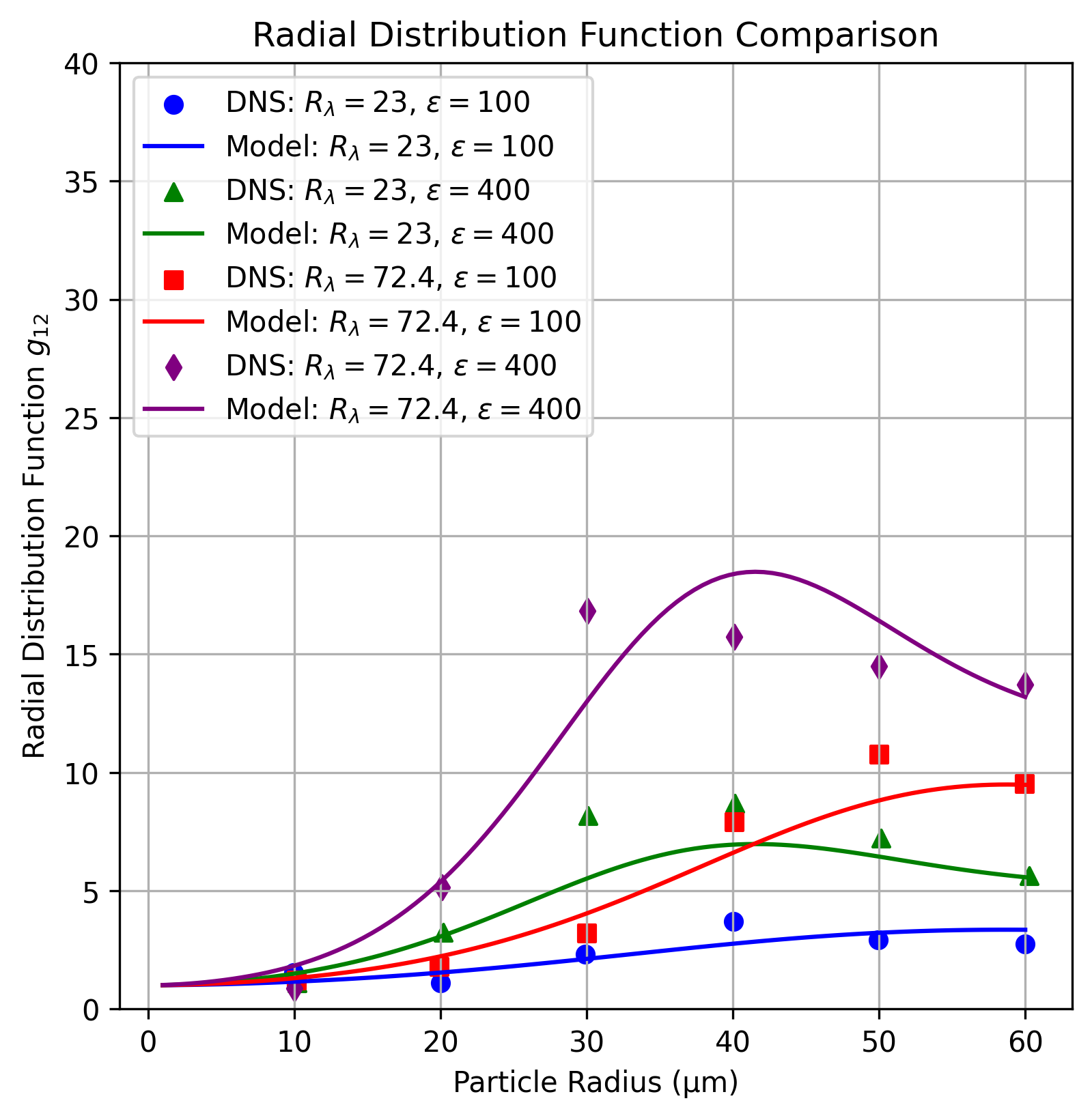
Summary
Section titled “Summary”Overall the comparison is good, and the curves are visually similar to Figure 16 in Ayala et al. (2008).
Explore this topic: Cloud-droplet collision kernels