

Explain a chamber spectrum using separate rate contributions
Explain a chamber spectrum using separate rate contributions
Section titled “Explain a chamber spectrum using separate rate contributions”A declining particle count can reflect dilution, wall deposition, or collisions. Which parts of the size distribution do those mechanisms change? This functional example calculates their instantaneous contributions and advances their sum for one hour. It helps distinguish a rate decomposition from a set of independent process-on/process-off simulations.
The initial two lognormal radius scales are 100 and 500 nm, with geometric standard deviations 1.3 and 1.5 and number densities 5×10¹⁰ and 5×10⁹ m⁻³. There are 250 radius bins from 10 nm–10 µm. The first figure shows number per volume per bin, not probability density. Density is 1000 kg m⁻³, temperature 293.15 K, and pressure 101325 Pa.
There is no condensation or chemistry. For the native container/runnable version and actual matched process combinations, see the wall-loss comparison.
Python · section 1
# In Colab uncomment the following command to install particula:# Install from the repository root: `python -m pip install -e ".[extra]"`import numpy as npimport particula as parfrom matplotlib import pyplot as pltPython · section 2
# Define initial simulation parametersmode = np.array([100e-9, 500e-9])  # Modal radius of the particles in metersgeometric_standard_deviation = np.array(    [1.3, 1.5])  # Geometric standard deviation of particle size distributionnumber_in_mode = (    np.array([5e4, 5e3]) * 1e6)  # Number of particles in each mode  1/m^3

# define the radius bins for the simulationradius_bins = np.logspace(-8, -5, 250)

# Create particle distribution using the defined parameters
concentration_pmf = par.particles.get_lognormal_pmf_distribution(    x_values=radius_bins,    mode=mode,    geometric_standard_deviation=geometric_standard_deviation,    number_of_particles=number_in_mode,)

# plot the initial particle distributionfig, ax = plt.subplots()ax.plot(    radius_bins, concentration_pmf, label="Initial distribution", marker=".")ax.set_xscale("log")ax.set_xlabel("Particle radius (m)")ax.set_ylabel(r"Particle Concentration (dN), $\dfrac{1}{m^{3}}$")plt.show()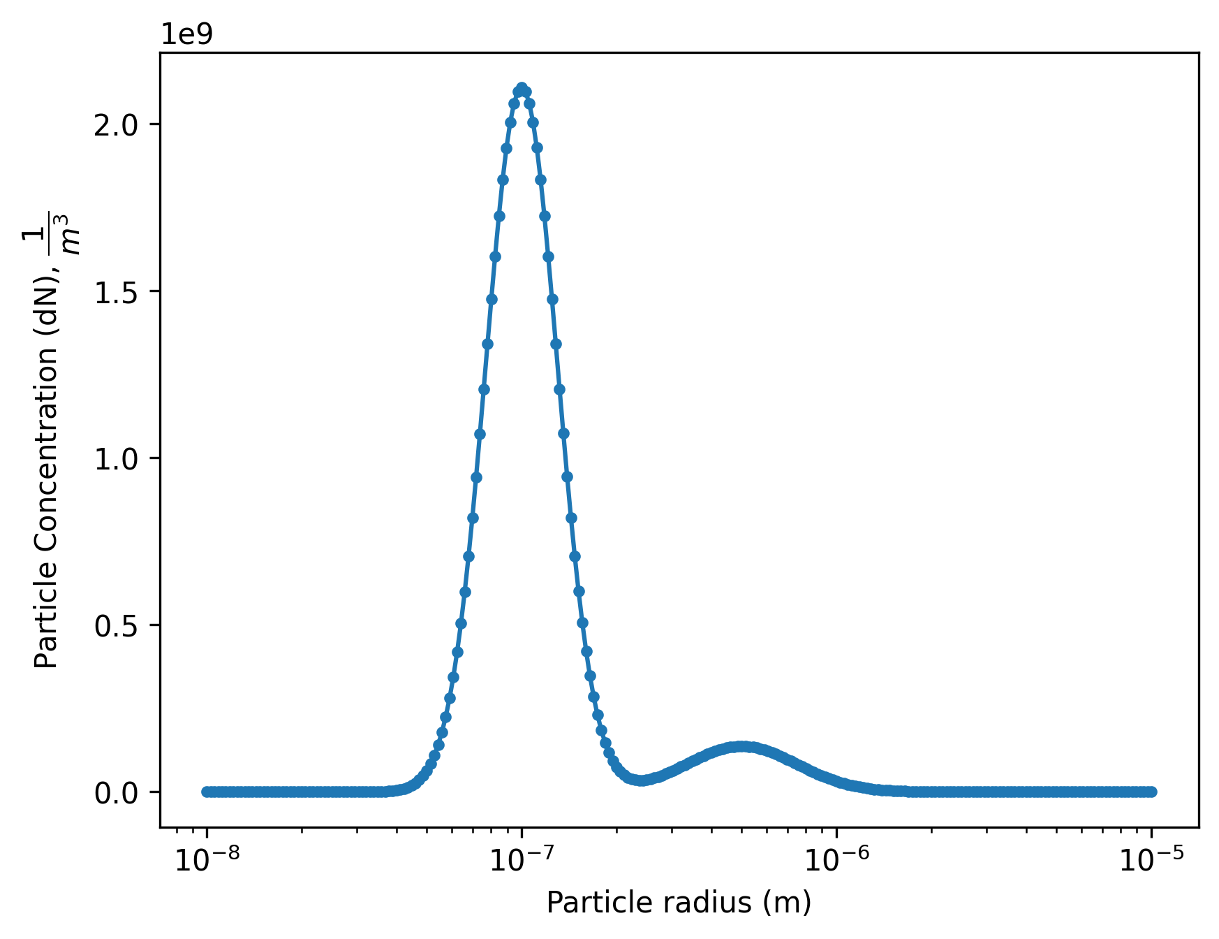
Compare rates at one common initial state
Section titled “Compare rates at one common initial state”Brownian coagulation contributes a gain and a loss term: its net rate can be positive at some radii even while total number falls. Dilution and wall loss remove particles. The dilution coefficient is flow/volume = 2×10⁻⁶ s⁻¹ for a 1 m³ well-mixed box. Wall loss uses a 1 × 1 × 1 m chamber and wall eddy parameter 0.1 s⁻¹.
The rate plot has units m⁻³ s⁻¹ per bin. A large absolute loss may reflect high abundance rather than a large fractional coefficient. Wall removal can be size selective through multiple transport mechanisms; it is not generically a process acting only on the largest particles.
Python · section 3
# coagulation rate
particle_mass = (    4 / 3 * np.pi * radius_bins**3 * 1000)  # mass of the particles in kg
kernel = np.asarray(    par.dynamics.get_brownian_kernel_via_system_state(        particle_radius=radius_bins,        particle_mass=particle_mass,        temperature=293.15,        pressure=101325,        alpha_collision_efficiency=1,    ),)coagulation_loss = par.dynamics.get_coagulation_loss_rate_discrete(    concentration=concentration_pmf,    kernel=kernel,)coagulation_gain = par.dynamics.get_coagulation_gain_rate_discrete(    radius=radius_bins,    concentration=concentration_pmf,    kernel=kernel,)coagulation_net = coagulation_gain - coagulation_loss
# dilution ratedilution_coefficent = par.dynamics.get_volume_dilution_coefficient(    volume=1,  # m^3    input_flow_rate=2 * 1e-6,  # m^3/s)dilution_loss = par.dynamics.get_dilution_rate(    coefficient=dilution_coefficent,    concentration=concentration_pmf,)
# wall loss ratechamber_wall_loss_rate = par.dynamics.get_rectangle_wall_loss_rate(    wall_eddy_diffusivity=0.1,    particle_radius=radius_bins,    particle_density=1000,    particle_concentration=concentration_pmf,    temperature=293.15,    pressure=101325,    chamber_dimensions=(1, 1, 1),  # m)
# plot ratesfig, ax = plt.subplots()ax.plot(    radius_bins,    coagulation_net,    label="Coagulation Net",)ax.plot(    radius_bins,    dilution_loss,    label="Dilution Loss",)ax.plot(    radius_bins,    chamber_wall_loss_rate,    label="Chamber Wall Loss",)ax.plot(    radius_bins,    coagulation_net + dilution_loss + chamber_wall_loss_rate,    label="Net Rate",    linestyle="--",)ax.set_xscale("log")# ax.set_yscale("log")ax.set_xlabel("Particle radius (m)")ax.set_ylabel(r"Rate $\dfrac{1}{m^{3} s^{1}}$")ax.grid()plt.legend()plt.show()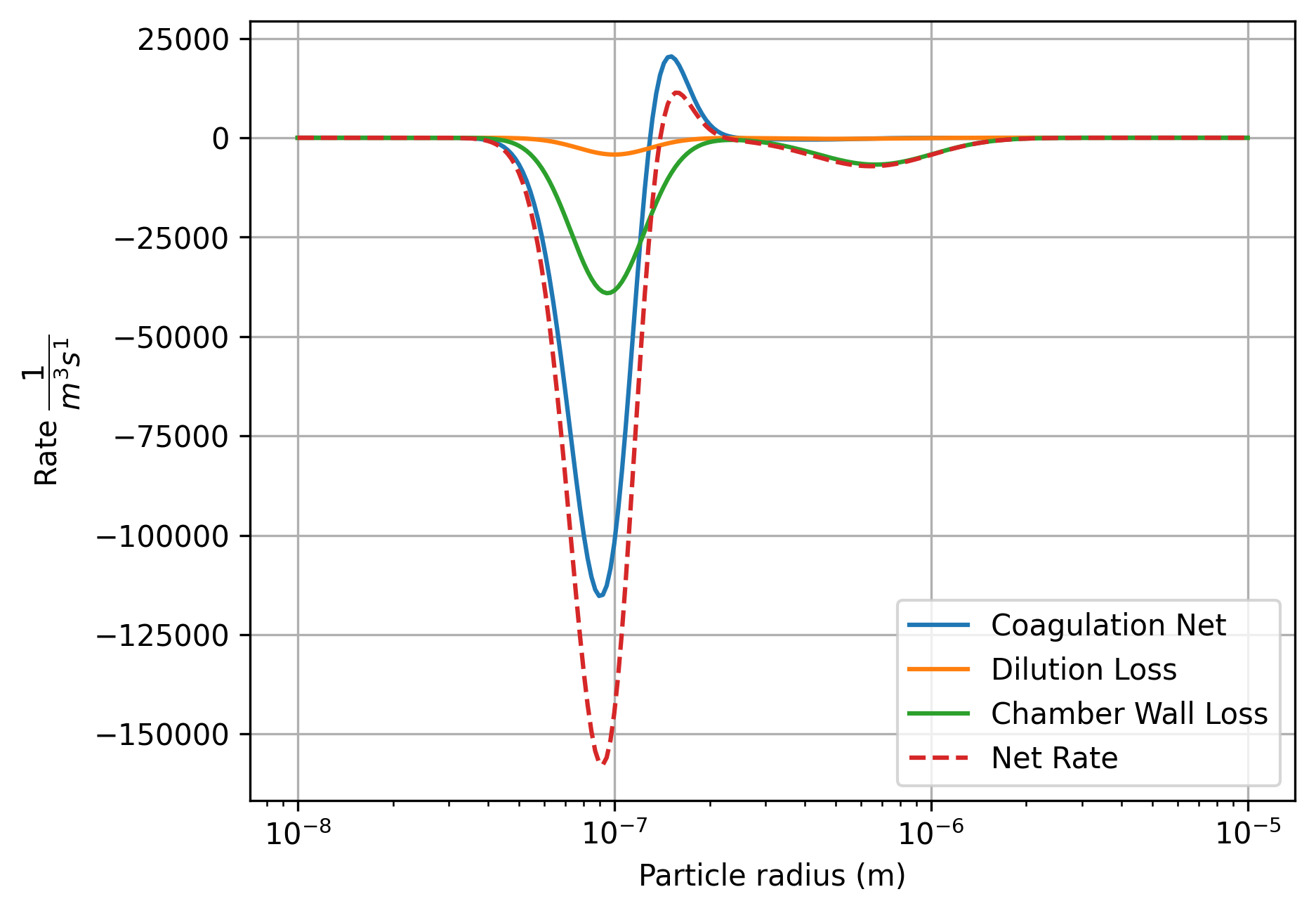
Integrate the combined model and retain each contribution
Section titled “Integrate the combined model and retain each contribution”The 1000 stored times span 0–3600 s, so there are 999 explicit Euler advances of about 3.604 s. The Brownian kernel stays fixed because grid, mass, and gas conditions are fixed; concentration-dependent rates are recomputed each step. The rate arrays record contributions evaluated at the preceding state.
Finite, nonnegative concentrations and nonincreasing total number are checked. These are useful admissibility checks, not a convergence demonstration. The functional route exposes the update directly, but shares underlying physical functions with other interfaces and is not an independent physics benchmark.
Python · section 4
# time stepstime_array = np.linspace(start=0, stop=3600, num=1000)dt = time_array[1] - time_array[0]
# create a matrix to store the particle distribution at each time stepconcentration_matrix = np.zeros((len(time_array), len(radius_bins)))coagulation_net_matrix = np.zeros((len(time_array), len(radius_bins)))dilution_loss_matrix = np.zeros((len(time_array), len(radius_bins)))chamber_wall_loss_rate_matrix = np.zeros((len(time_array), len(radius_bins)))
# set the initial concentrationconcentration_matrix[0, :] = concentration_pmf
kernel = np.asarray(    par.dynamics.get_brownian_kernel_via_system_state(        particle_radius=radius_bins,        particle_mass=particle_mass,        temperature=293.15,        pressure=101325,        alpha_collision_efficiency=1,    ))# iterate over the time stepsfor i in range(1, len(time_array)):    # calculate the coagulation rate    coagulation_loss = par.dynamics.get_coagulation_loss_rate_discrete(        concentration=concentration_matrix[i - 1, :],        kernel=kernel,    )    coagulation_gain = par.dynamics.get_coagulation_gain_rate_discrete(        radius=radius_bins,        concentration=concentration_matrix[i - 1, :],        kernel=kernel,    )    coagulation_net = coagulation_gain - coagulation_loss
    # calculate the dilution rate    dilution_coefficent = par.dynamics.get_volume_dilution_coefficient(        volume=1,  # m^3        input_flow_rate=2 * 1e-6,  # m^3/s    )    dilution_loss = par.dynamics.get_dilution_rate(        coefficient=dilution_coefficent,        concentration=concentration_matrix[i - 1, :],    )
    # calculate the wall loss rate    chamber_wall_loss_rate = par.dynamics.get_rectangle_wall_loss_rate(        wall_eddy_diffusivity=0.1,        particle_radius=radius_bins,        particle_density=1000,        particle_concentration=concentration_matrix[i - 1, :],        temperature=293.15,        pressure=101325,        chamber_dimensions=(1, 1, 1),  # m    )
    # update the concentration matrix    concentration_matrix[i, :] = (        concentration_matrix[i - 1, :]        + (coagulation_net + dilution_loss + chamber_wall_loss_rate) * dt    )
    # update the rate matrices    coagulation_net_matrix[i, :] = coagulation_net    dilution_loss_matrix[i, :] = dilution_loss    chamber_wall_loss_rate_matrix[i, :] = chamber_wall_loss_rate
assert np.all(np.isfinite(concentration_matrix))assert np.all(concentration_matrix >= 0)assert np.all(np.diff(concentration_matrix.sum(axis=1)) <= 0)print("Done")DoneRead evolution without inventing missing control cases
Section titled “Read evolution without inventing missing control cases”The spectrum plot compares the initial and final states of the combined model; no midpoint spectrum is plotted. The following panel compares initial rate contributions with those evaluated at the last pre-update state, approximately 3596.4 s. It therefore shows how the evolving population changes each rate, not a set of separate coagulation-only or dilution-only trajectories.
Redistribution toward larger bins can come from coagulation, while external losses lower airborne abundance. The combined spectrum alone does not assign a unique fraction of total loss to each mechanism.
Python · section 5
# Plotting the simulation results# Adjusting the figure size for better clarityfig, ax = plt.subplots(1, 1, figsize=[8, 6])
# plot the initial particle distributionax.plot(    radius_bins,    concentration_matrix[0, :],    label="Initial distribution",)# plot the final particle distributionax.plot(    radius_bins,    concentration_matrix[-1, :],    label="Final distribution",)ax.set_xscale("log")ax.set_xlabel("Particle radius (m)")ax.set_ylabel(r"Particle Concentration (dN), $\dfrac{1}{m^{3}}$")plt.legend()plt.show()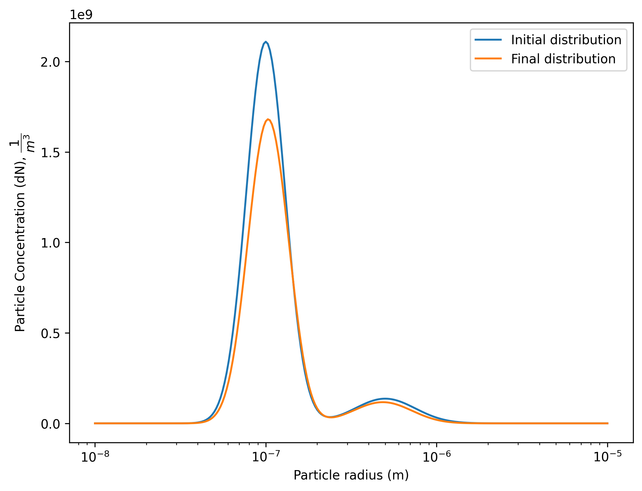
Python · section 6
# plot the Initial and Final ratesfig, ax = plt.subplots()ax.plot( radius_bins, coagulation_net_matrix[1, :], color="tab:blue", label="Initial Coagulation Net",)ax.plot( radius_bins, dilution_loss_matrix[1, :], color="tab:orange", label="Initial Dilution Loss",)ax.plot( radius_bins, chamber_wall_loss_rate_matrix[1, :], color="tab:green", label="Initial Chamber Wall Loss",)ax.plot( radius_bins, coagulation_net_matrix[-1, :], color="tab:blue", label="Final Coagulation Net", linestyle="--",)ax.plot( radius_bins, dilution_loss_matrix[-1, :], color="tab:orange", label="Final Dilution Loss", linestyle="--",)ax.plot( radius_bins, chamber_wall_loss_rate_matrix[-1, :], color="tab:green", label="Final Chamber Wall Loss", linestyle="--",)ax.set_xscale("log")ax.set_xlabel("Particle radius (m)")ax.set_ylabel(r"Rate $\dfrac{1}{m^{3} s^{1}}$")ax.grid()plt.legend()plt.show()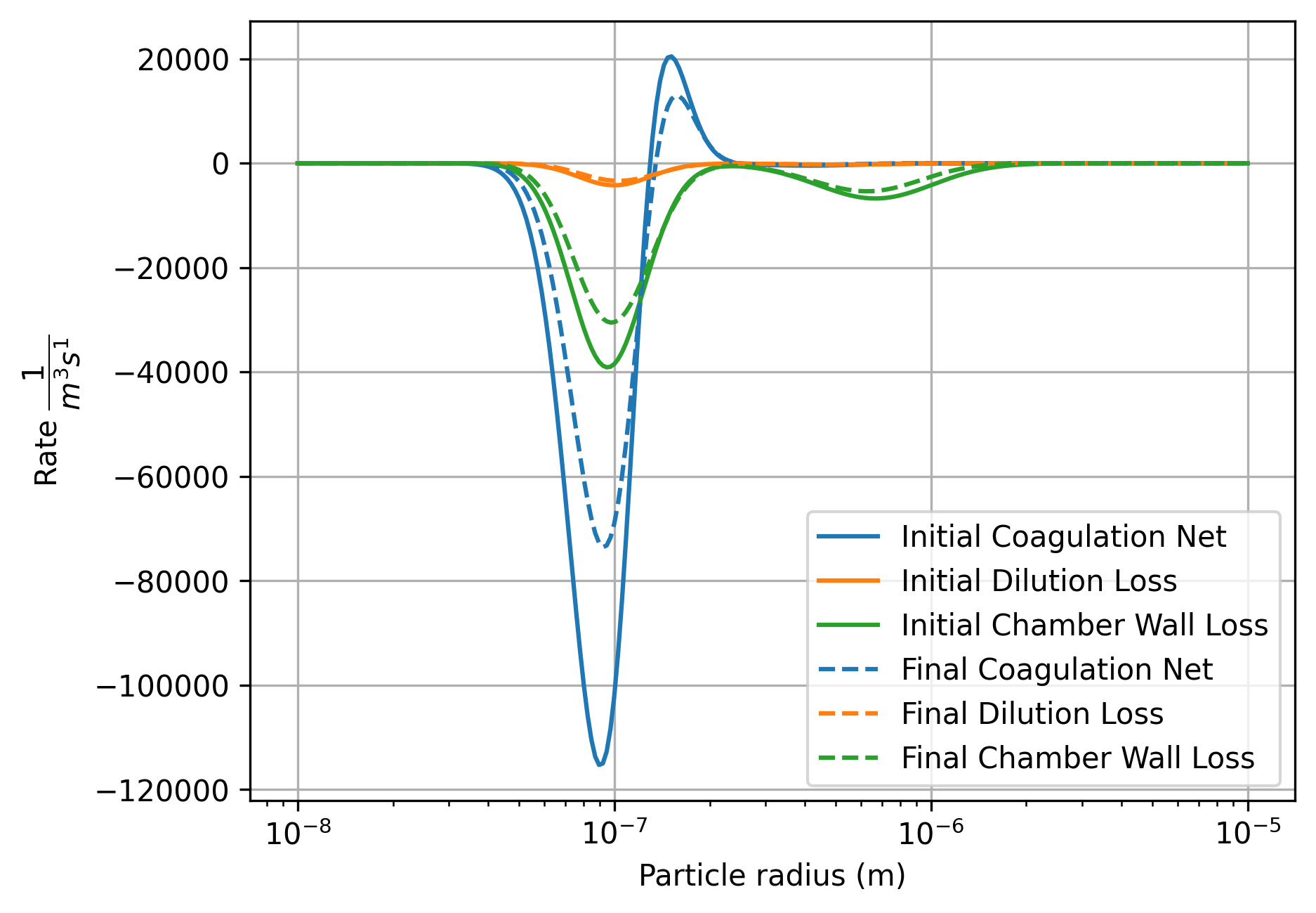
Turn a rate decomposition into a causal comparison
Section titled “Turn a rate decomposition into a causal comparison”This run demonstrates a finite, nonnegative combined trajectory and exposes its three rate contributions. It does not compare with experimental observations or establish that one mechanism is required by data. No isolated-process simulation is performed here.
To test which mechanism controls a measured chamber decay, repeat from the same initial spectrum with one process disabled at a time. Track number, airborne mass, and cumulative external removal; refine timestep and radius grid to separate numerical drift from physical loss. Compare those predictions with size-resolved measurements and independent flow/geometry estimates before attributing an observed change to wall loss or coagulation.
Explore this topic: Wall deposition