

Brownian coagulation in a PMF population
Python · section 1
"""Showcase a PMF-based Brownian coagulation example.
Builds a lognormal PMF aerosol, configures Brownian coagulation with``distribution_type="discrete"``, runs a short guarded step, and plots PMFconcentration before/after execution to visualize redistribution. Designedfor quick execution with a small grid and modest sub-steps.
Example:    Run the script to generate before/after concentration curves for a    discrete PMF aerosol using the public ``par.dynamics`` API."""
'Showcase a PMF-based Brownian coagulation example.\n\nBuilds a lognormal PMF aerosol, configures Brownian coagulation with\n``distribution_type="discrete"``, runs a short guarded step, and plots PMF\nconcentration before/after execution to visualize redistribution. Designed\nfor quick execution with a small grid and modest sub-steps.\n\nExample:\n Run the script to generate before/after concentration curves for a\n discrete PMF aerosol using the public ``par.dynamics`` API.\n'Brownian coagulation in a PMF population
Section titled “Brownian coagulation in a PMF population”How can collisions reduce particle number while transferring material toward larger sizes? This example follows a single-material aerosol through two hours of Brownian coagulation. The central reading skill is distinguishing number loss from material loss: a collision merges particles rather than removing their constituent mass.
Here the stored concentration has units m⁻³ per bin. To obtain total number density, sum the bin concentrations. Review distribution measures before comparing this plot with another representation.
Python · section 2
# In Colab uncomment the following command to install particula:# Install from the repository root: `python -m pip install -e ".[extra]"`import matplotlib.pyplot as pltimport numpy as npimport particula as parEstablish the population and its measure
Section titled “Establish the population and its measure”The 150 radius nodes span 10 nm–10 µm. A lognormal radius scale of 80 nm,
geometric standard deviation 1.5, and specified total number density 10¹⁰ m⁻³
set the initial population; density is 1000 kg m⁻³. The parameter named mode
is the lognormal scale, not the peak of every possible plotted measure.
Temperature and pressure are held at 298.15 K and 101325 Pa. The zero-concentration carrier satisfies the gas-container shape contract; coagulation does not consume it. No condensation, dilution, charging, or wall loss is included.
Python · section 3
# Radius bins (log-spaced, extended to 10 microns for visibility)radius_bins = np.logspace(-8, -5, 150)  # m (10 nm to 10 um)
# Lognormal PMF (concentration per bin) - higher concentration for visible changeconcentration_pmf = par.particles.get_lognormal_pmf_distribution(    x_values=radius_bins,    mode=np.array([80e-9]),    geometric_standard_deviation=np.array([1.5]),    number_of_particles=np.array(        [1e10]    ),  # m^-3 total (increased for visibility))
# Native ambient environment. GasData requires a species axis, so a# zero-concentration, non-partitioning carrier fills that axis. Coagulation# does not consume it; ambient pressure is specified independently.environment = par.gas.EnvironmentData(    temperature=np.array([298.15]),    pressure=np.array([101325.0]),    saturation_ratio=np.zeros((1, 1)),)gas = par.gas.GasData(    name=["carrier"],    molar_mass=np.array([0.02897]),    partitioning=np.array([False]),    concentration=np.zeros((1, 1)),)particles_pmf = par.particles.create_particle_data_from_radii(    radii=radius_bins,    concentration=concentration_pmf,    distribution_type="discrete",    density=1000.0,)pmf_aerosol = par.Aerosol(    particles=particles_pmf,    gas=gas,    environment=environment,)
Connect collision physics to the stored distribution
Section titled “Connect collision physics to the stored distribution”The Brownian strategy supplies size-dependent collision rates. Its distribution
setting must agree with the particle container: bin totals and densities per
radius require different numerical operations. The Coagulation wrapper
advances the supplied aerosol in place, so preserve a copy for an independent
control.
Python · section 4
coagulation_strategy = (    par.dynamics.BrownianCoagulationBuilder()    .set_distribution_type("discrete")    .build())coagulation_process = par.dynamics.Coagulation(    coagulation_strategy=coagulation_strategy)
print(coagulation_process)
<particula.dynamics.particle_process.Coagulation object at 0x7fddaf1531a0>Track two one-hour advances
Section titled “Track two one-hour advances”Each call advances 3600 s with 100 substeps. The snapshots therefore represent initial, one-hour, and two-hour states. The finite/nonnegative checks reject invalid concentrations, while the printed relative mass change diagnoses material drift on this finite grid. These checks answer different questions: nonnegative output alone does not establish conservation or convergence.
For mass density, weight by the spherical single-particle mass before you sum the bin concentrations. Keep that integration convention consistent between snapshots.
Python · section 5
# Set up time and sub-steps for the coagulation process# Longer time span for visible coagulation effecttime_step = 3600  # 1 hour per stepsub_steps = 100
radii = pmf_aerosol.particles.radii[0]pmf_before = np.copy(pmf_aerosol.particles.concentration[0])
# Perform coagulation process for step 1pmf_aerosol = coagulation_process.execute(    pmf_aerosol, time_step=time_step, sub_steps=sub_steps)radii_after_step_1 = pmf_aerosol.particles.radii[0]pmf_after_step_1 = np.copy(pmf_aerosol.particles.concentration[0])
# Perform coagulation process for step 2pmf_aerosol = coagulation_process.execute(    pmf_aerosol, time_step=time_step, sub_steps=sub_steps)radii_after_step_2 = pmf_aerosol.particles.radii[0]pmf_after_step_2 = np.copy(pmf_aerosol.particles.concentration[0])
Python · section 6
# Independently account for material mass; PDF values require radius integration.bin_mass = 4.0 / 3.0 * np.pi * radius_bins**3 * 1000.0mass_history = np.array( [ np.sum(values * bin_mass) for values in (pmf_before, pmf_after_step_1, pmf_after_step_2) ])print("Relative material mass drift:", mass_history / mass_history[0] - 1)assert np.all(np.isfinite(pmf_after_step_2))assert np.all(pmf_after_step_2 >= 0)Relative material mass drift: [ 0. -0.0011476 -0.00225778]Read redistribution rather than peak height alone
Section titled “Read redistribution rather than peak height alone”The vertical axis is m⁻³ per bin; a lower peak is not by itself the fraction of particles lost. Compare the small-radius depletion and larger-radius redistribution, then use the appropriate total-number diagnostic. The logarithmic horizontal axis changes visual spacing, not the definition of the stored measure.
Python · section 7
fig, ax = plt.subplots(figsize=(8, 5))ax.plot(radii, pmf_before, label="Initial", color="tab:blue")ax.plot( radii_after_step_1, pmf_after_step_1, label="After step 1", color="tab:orange",)ax.plot( radii_after_step_2, pmf_after_step_2, label="After step 2", color="tab:green",)ax.set_xscale("log")ax.set_xlim(1e-8, 1e-5) # 10 nm to 10 umax.set_xlabel("Particle radius (m)")ax.set_ylabel(r"Number concentration ($m^{-3}$)")ax.set_title("PMF coagulation (Brownian, discrete)")ax.legend()ax.grid(alpha=0.3)plt.show()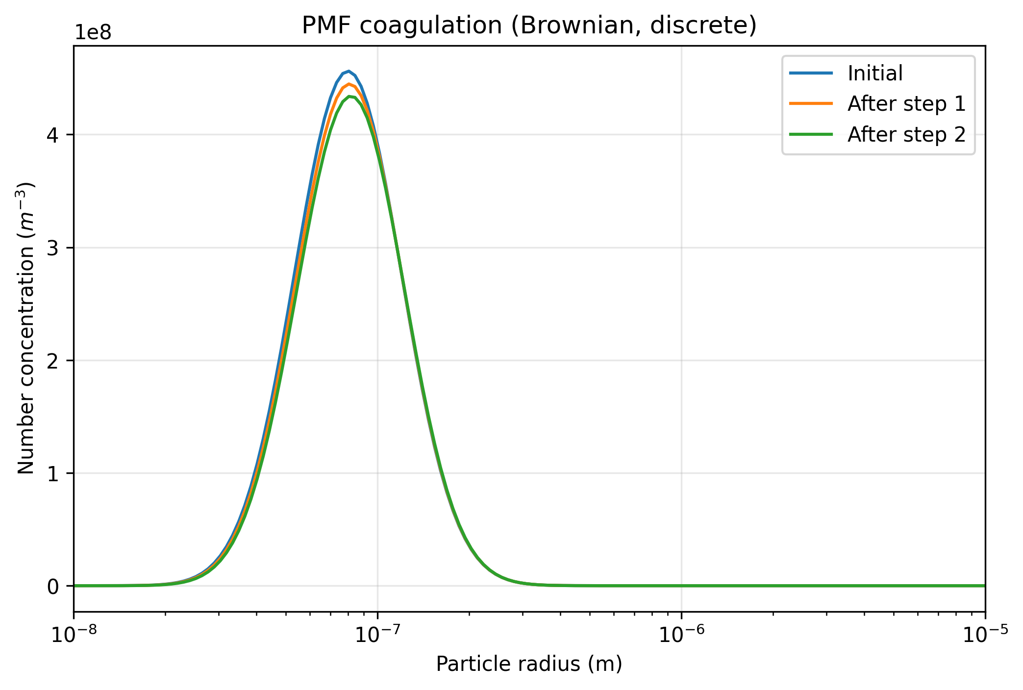
Bound the numerical conclusion
Section titled “Bound the numerical conclusion”The explicitly generated input distribution is retained by native construction. Finite-grid coagulation need not conserve mass exactly: truncation and numerical redistribution can affect the result. This one grid and one substep choice do not measure those errors independently.
From this curve to a defensible comparison
Section titled “From this curve to a defensible comparison”This calculation connects collision-driven number loss to evolving size occupancy. To determine whether the predicted loss is robust, vary radius-grid resolution and extent separately from substep size; compare total number and mass drift at the same physical times.
Next use the PMF/PDF comparison to place both representations in common units. For a composition-resolved research question, explore individual-particle coagulation and add independent stochastic realizations before attributing small differences to the representation.
Explore this topic: Binned populations