

Does particle-number decay depend on representation?
Python · section 1
"""Compare time evolution of total number concentration across coagulation.
Builds PMF, PDF, and particle-resolved aerosols with equivalent lognormaldistributions, configures Brownian coagulation for each representation,and tracks total number concentration over time. Plots the decay of particlenumber for all three approaches on the same axes to compare how eachrepresentation tracks coagulation-driven particle loss.
Example:    Run the script to visualize how total number concentration decreases    over time for PMF, PDF, and particle-resolved coagulation representations."""
'Compare time evolution of total number concentration across coagulation.\n\nBuilds PMF, PDF, and particle-resolved aerosols with equivalent lognormal\ndistributions, configures Brownian coagulation for each representation,\nand tracks total number concentration over time. Plots the decay of particle\nnumber for all three approaches on the same axes to compare how each\nrepresentation tracks coagulation-driven particle loss.\n\nExample:\n Run the script to visualize how total number concentration decreases\n over time for PMF, PDF, and particle-resolved coagulation representations.\n'Does particle-number decay depend on representation?
Section titled “Does particle-number decay depend on representation?”A size spectrum can look different simply because its vertical axis differs. Total number density provides a shared diagnostic for PMF, PDF, and sampled particle populations. Here all three use the same nominal lognormal population and Brownian mechanism over two hours.
The aim is to construct a fair comparison and interpret its limits. Read the PMF/PDF unit comparison first if sums, integrals, and counts per volume are not yet distinct.
Python · section 2
# In Colab uncomment the following command to install particula:# Install from the repository root: `python -m pip install -e ".[extra]"`import matplotlib.pyplot as pltimport numpy as npimport particula as parfrom scipy.integrate import trapezoidMatch a target population, not every individual radius
Section titled “Match a target population, not every individual radius”The target lognormal radius scale is 80 nm, geometric standard deviation 1.5, and number density 10¹⁰ m⁻³. PMF and PDF use 150 nodes from 10 nm to 10 µm; the particle population samples the same nominal law. Finite quadrature and sampling mean their initial size distributions are not identical realizations. Density is 1000 kg m⁻³ at fixed 298.15 K and 101325 Pa.
Python · section 3
# Shared radius bins for PMF and PDFradius_bins = np.logspace(-8, -5, 150)  # m (10 nm to 10 um)
# Lognormal parameters (shared across all representations)mode = np.array([80e-9])  # 80 nmgsd = np.array([1.5])number_conc = np.array([1e10])  # m^-3 total
# Native ambient environment. GasData requires a species axis, so a# zero-concentration, non-partitioning carrier fills that axis. Coagulation# does not consume it; ambient pressure is specified independently.environment = par.gas.EnvironmentData(    temperature=np.array([298.15]),    pressure=np.array([101325.0]),    saturation_ratio=np.zeros((1, 1)),)gas = par.gas.GasData(    name=["carrier"],    molar_mass=np.array([0.02897]),    partitioning=np.array([False]),    concentration=np.zeros((1, 1)),)
Bin totals: sum to obtain abundance
Section titled “Bin totals: sum to obtain abundance”The discrete concentration stores m⁻³ per bin. Summing the initialized array gives the PMF number density against which the sampled population is matched.
Python · section 4
# PMF distribution (number per bin)concentration_pmf = par.particles.get_lognormal_pmf_distribution(    x_values=radius_bins,    mode=mode,    geometric_standard_deviation=gsd,    number_of_particles=number_conc,)
# Build PMF particle representationparticles_pmf = par.particles.create_particle_data_from_radii(    radii=radius_bins,    concentration=concentration_pmf,    distribution_type="discrete",    density=1000.0,)
aerosol_pmf = par.Aerosol(    particles=particles_pmf, gas=gas.copy(), environment=environment.copy())print(f"PMF initial total: {concentration_pmf.sum():.2e} m^-3")
PMF initial total: 1.00e+10 m^-3Radius density: integrate to obtain abundance
Section titled “Radius density: integrate to obtain abundance”The continuous concentration stores m⁻⁴. Its total is a trapezoidal integral over radius, not the unweighted sum of stored values. Retain this distinction at every time point, including normalization.
Python · section 5
# PDF distribution (number per unit size)concentration_pdf = par.particles.get_lognormal_pdf_distribution(    x_values=radius_bins,    mode=mode,    geometric_standard_deviation=gsd,    number_of_particles=number_conc,)
# Build PDF particle representationparticles_pdf = par.particles.create_particle_data_from_radii(    radii=radius_bins,    concentration=concentration_pdf,    distribution_type="continuous_pdf",    density=1000.0,)
aerosol_pdf = par.Aerosol(    particles=particles_pdf, gas=gas.copy(), environment=environment.copy())pdf_total = trapezoid(concentration_pdf, x=radius_bins)print(f"PDF initial total: {pdf_total:.2e} m^-3")
PDF initial total: 1.00e+10 m^-3Sampled particles: set the physical volume
Section titled “Sampled particles: set the physical volume”The 50,000 sampled particles have unit represented counts. Volume is chosen as sample count divided by the actual initial PMF number density, matching abundance without pretending the samples occupy identical radius nodes. The initial count-weighted material inventory is retained for a conservation check.
Python · section 6
# Sample radii from the same lognormal distribution# Match the actual PMF aerosol concentration (after builder processing)pmf_initial_concentration = aerosol_pmf.particles.number_density[0]n_samples = 50_000
np.random.seed(42)radii_sample = par.particles.get_lognormal_sample_distribution(    mode=mode,    geometric_standard_deviation=gsd,    number_of_particles=np.array([1.0]),  # relative weighting    number_of_samples=n_samples,)
# Volume is set so total concentration matches PMF initial# concentration = n_particles / volume -> volume = n_particles / concentrationsample_volume = len(radii_sample) / pmf_initial_concentration
# Compute mass from radius and densitydensity = np.array([1_000.0])mass_sample = 4 / 3 * np.pi * radii_sample**3 * density
# Unit count weights and the physical volume establish number density.particles_resolved = par.particles.create_resolved_particle_data(    masses=mass_sample,    density=density,    volume=sample_volume,)aerosol_resolved = par.Aerosol(    particles=particles_resolved,    gas=gas.copy(),    environment=environment.copy(),)initial_resolved_inventory = np.sum(    particles_resolved.masses * particles_resolved.concentration[..., None],    axis=1,)print(f"Particle-resolved initial count: {len(radii_sample)} particles")print(    f"  -> concentration: {aerosol_resolved.particles.number_density[0]:.2e} m^-3")
Particle-resolved initial count: 50000 particles
-> concentration: 1.00e+10 m^-3Use one mechanism with three numerical representations
Section titled “Use one mechanism with three numerical representations”Each wrapper selects Brownian coagulation and the storage-appropriate distribution type. The zero-concentration carrier is structural, not a source or sink. With no other processes, declining particle number is attributable to coagulation.
Python · section 7
# PMF coagulation (discrete)coagulation_pmf = par.dynamics.Coagulation(    coagulation_strategy=(        par.dynamics.BrownianCoagulationBuilder()        .set_distribution_type("discrete")        .build()    ))
# PDF coagulation (continuous)coagulation_pdf = par.dynamics.Coagulation(    coagulation_strategy=(        par.dynamics.BrownianCoagulationBuilder()        .set_distribution_type("continuous_pdf")        .build()    ))
# Particle-resolved coagulationcoagulation_resolved = par.dynamics.Coagulation(    coagulation_strategy=(        par.dynamics.BrownianCoagulationBuilder()        .set_distribution_type("particle_resolved")        .build()    ))
print("PMF:", coagulation_pmf)print("PDF:", coagulation_pdf)print("Resolved:", coagulation_resolved)
PMF: <particula.dynamics.particle_process.Coagulation object at 0x7fd7e7104e90>
PDF: <particula.dynamics.particle_process.Coagulation object at 0x7fd7a774bb60>
Resolved: <particula.dynamics.particle_process.Coagulation object at 0x7fd7a6fc0bc0>Follow a common clock and diagnostic
Section titled “Follow a common clock and diagnostic”Twelve 600 s advances, each with 50 substeps, give two hours of evolution plus the initial state. PMF and particle-resolved totals use native number density; the PDF is integrated over radius. The resolved assertion checks material inventory at every step, not just the endpoint. No corresponding assertion here establishes exact mass conservation for the finite-grid methods.
Python · section 8
# Time parameterstime_step = 600  # seconds (10 minutes)sub_steps = 50n_steps = 12  # 12 steps = 2 hours total
# Time array for plottingtimes = np.arange(0, (n_steps + 1) * time_step, time_step)  # 0 to 7200 s
# Storage for number concentrations# PMF and Resolved: native number_density respects density/count semantics# PDF: must integrate since concentration is per unit size (m^-4)number_pmf = [aerosol_pmf.particles.number_density[0]]number_pdf = [trapezoid(aerosol_pdf.particles.concentration[0], x=radius_bins)]number_resolved = [aerosol_resolved.particles.number_density[0]]
print(    f"Initial: PMF={number_pmf[0]:.2e}, PDF={number_pdf[0]:.2e}, "    f"Resolved={number_resolved[0]:.2e}")
print(f"Running {n_steps} steps of {time_step}s each ({sub_steps} sub-steps)")print(f"Total simulation time: {n_steps * time_step / 3600:.1f} hours")
Initial: PMF=1.00e+10, PDF=1.00e+10, Resolved=1.00e+10
Running 12 steps of 600s each (50 sub-steps)
Total simulation time: 2.0 hoursPython · section 9
# Run time evolution for all three representationsfor step in range(n_steps):    # PMF coagulation    aerosol_pmf = coagulation_pmf.execute(        aerosol_pmf, time_step=time_step, sub_steps=sub_steps    )    number_pmf.append(aerosol_pmf.particles.number_density[0])
    # PDF coagulation    aerosol_pdf = coagulation_pdf.execute(        aerosol_pdf, time_step=time_step, sub_steps=sub_steps    )    number_pdf.append(        trapezoid(aerosol_pdf.particles.concentration[0], x=radius_bins)    )
    # Particle-resolved coagulation    aerosol_resolved = coagulation_resolved.execute(        aerosol_resolved, time_step=time_step, sub_steps=sub_steps    )    number_resolved.append(aerosol_resolved.particles.number_density[0])    np.testing.assert_allclose(        np.sum(            aerosol_resolved.particles.masses            * aerosol_resolved.particles.concentration[..., None],            axis=1,        ),        initial_resolved_inventory,        rtol=1e-12,        atol=1e-30,    )
    print(        f"Step {step + 1}/{n_steps}: "        f"PMF={number_pmf[-1]:.2e}, "        f"PDF={number_pdf[-1]:.2e}, "        f"Resolved={number_resolved[-1]:.2e}"    )
# Convert to arrays for plottingnumber_pmf = np.array(number_pmf)number_pdf = np.array(number_pdf)number_resolved = np.array(number_resolved)
Step 1/12: PMF=9.96e+09, PDF=9.96e+09, Resolved=9.96e+09Step 2/12: PMF=9.91e+09, PDF=9.92e+09, Resolved=9.91e+09Step 3/12: PMF=9.87e+09, PDF=9.88e+09, Resolved=9.87e+09Step 4/12: PMF=9.83e+09, PDF=9.83e+09, Resolved=9.83e+09Step 5/12: PMF=9.79e+09, PDF=9.79e+09, Resolved=9.79e+09Step 6/12: PMF=9.75e+09, PDF=9.75e+09, Resolved=9.76e+09Step 7/12: PMF=9.71e+09, PDF=9.71e+09, Resolved=9.72e+09Step 8/12: PMF=9.67e+09, PDF=9.68e+09, Resolved=9.68e+09Step 9/12: PMF=9.63e+09, PDF=9.64e+09, Resolved=9.64e+09Step 10/12: PMF=9.59e+09, PDF=9.60e+09, Resolved=9.60e+09Step 11/12: PMF=9.55e+09, PDF=9.56e+09, Resolved=9.56e+09Step 12/12: PMF=9.51e+09, PDF=9.52e+09, Resolved=9.51e+09Compare absolute abundance first
Section titled “Compare absolute abundance first”The first plot shows number density in m⁻³. Inspect initial alignment as well as subsequent decay; equal normalized slopes could hide unequal physical abundances. Collision frequency depends on the population available to collide, so a concentration mismatch would change the experiment itself.
Python · section 10
fig, ax = plt.subplots(figsize=(10, 6))
ax.plot(    times,    number_pmf,    "o-",    color="tab:blue",    label="PMF (discrete)",    markersize=6,)ax.plot(    times,    number_pdf,    "s-",    color="tab:orange",    label="PDF (continuous)",    markersize=6,)ax.plot(    times,    number_resolved,    "^-",    color="tab:green",    label="Particle-resolved",    markersize=6,)
ax.set_xlabel("Time (s)")ax.set_ylabel(r"Total number concentration (m$^{-3}$)")ax.set_title("Coagulation time evolution: PMF vs PDF vs Particle-resolved")ax.legend()ax.grid(alpha=0.3)
# Add secondary x-axis for time in hoursax2 = ax.twiny()ax2.set_xlim(ax.get_xlim())ax2.set_xticks(np.arange(0, 7201, 1800))ax2.set_xticklabels([f"{t / 3600:.1f}" for t in np.arange(0, 7201, 1800)])ax2.set_xlabel("Time (hours)")
plt.tight_layout()plt.show()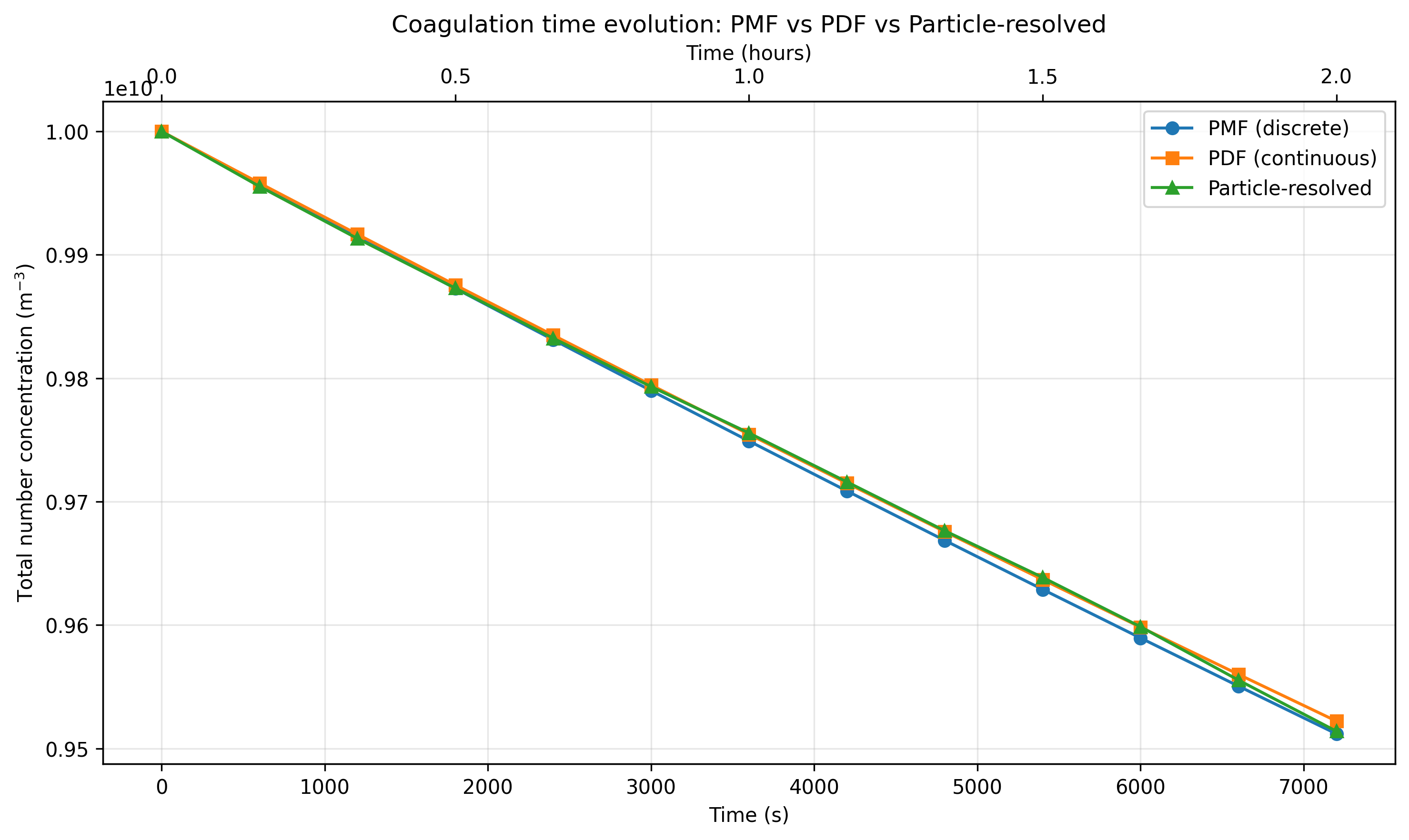
Then compare the fraction remaining
Section titled “Then compare the fraction remaining”Dividing by each initial number removes small initialization offsets from the display. The saved run reports about 95.1% remaining for PMF and 95.2% for PDF and resolved particles after two hours. Those rounded values show similar number decay for this workload, not identical spectra or validated accuracy. The resolved curve is one stochastic realization, with no uncertainty band.
Python · section 11
# Normalize to initial concentration for easier comparisonfig, ax = plt.subplots(figsize=(10, 6))
ax.plot(    times,    number_pmf / number_pmf[0],    "o-",    color="tab:blue",    label="PMF (discrete)",    markersize=6,)ax.plot(    times,    number_pdf / number_pdf[0],    "s-",    color="tab:orange",    label="PDF (continuous)",    markersize=6,)ax.plot(    times,    number_resolved / number_resolved[0],    "^-",    color="tab:green",    label="Particle-resolved",    markersize=6,)
ax.set_xlabel("Time (s)")ax.set_ylabel("Normalized number concentration (N/N0)")ax.set_title("Normalized coagulation decay: PMF vs PDF vs Particle-resolved")ax.legend()ax.grid(alpha=0.3)
# Add secondary x-axis for time in hoursax2 = ax.twiny()ax2.set_xlim(ax.get_xlim())ax2.set_xticks(np.arange(0, 7201, 1800))ax2.set_xticklabels([f"{t / 3600:.1f}" for t in np.arange(0, 7201, 1800)])ax2.set_xlabel("Time (hours)")
plt.tight_layout()plt.show()
# Print final valuesprint("\nFinal concentrations:")pmf_pct = 100 * number_pmf[-1] / number_pmf[0]pdf_pct = 100 * number_pdf[-1] / number_pdf[0]res_pct = 100 * number_resolved[-1] / number_resolved[0]print(f"  PMF: {number_pmf[-1]:.2e} m^-3 ({pmf_pct:.1f}% remaining)")print(f"  PDF: {number_pdf[-1]:.2e} m^-3 ({pdf_pct:.1f}% remaining)")print(f"  Resolved: {number_resolved[-1]:.2e} m^-3 ({res_pct:.1f}% remaining)")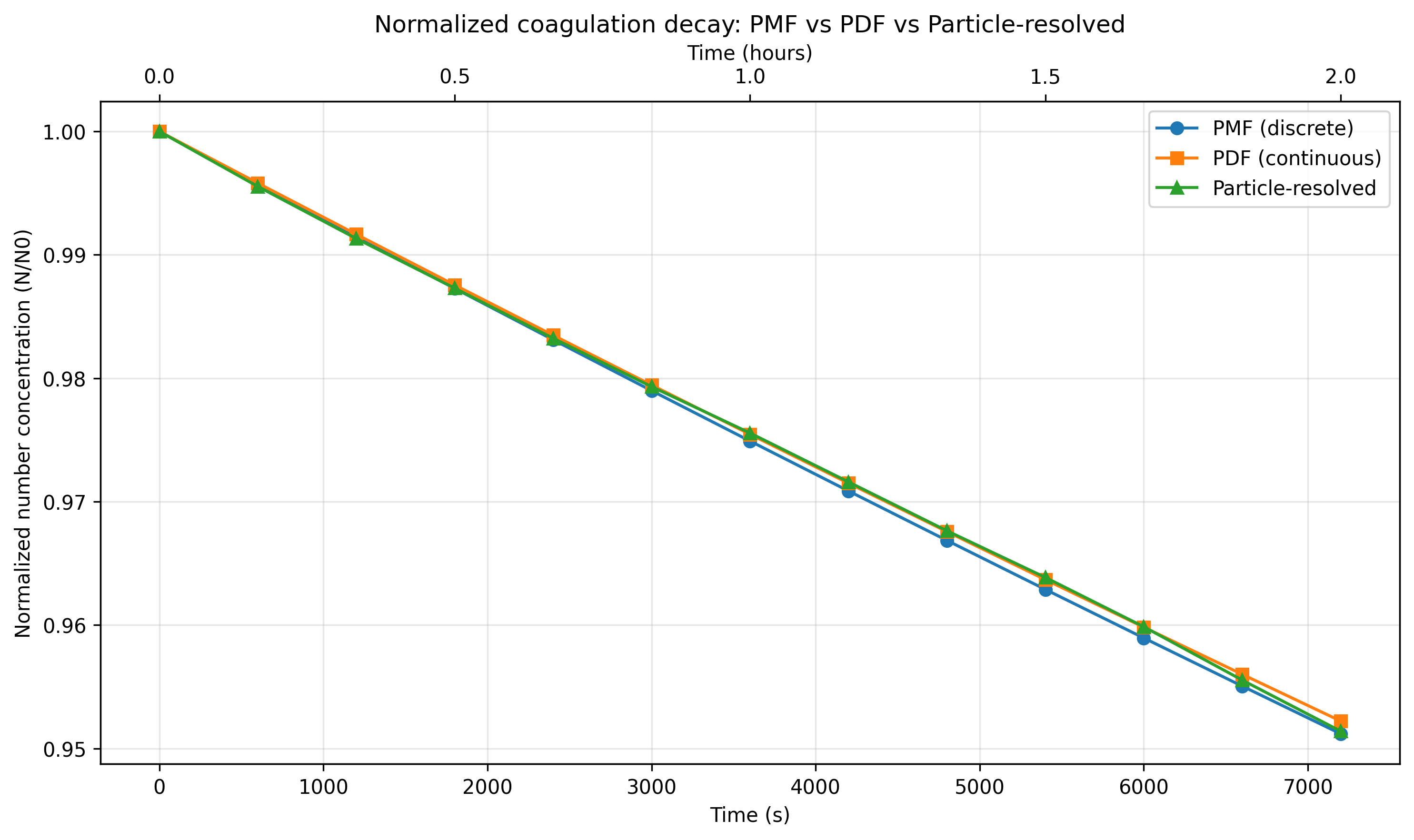
Final concentrations:
  PMF: 9.51e+09 m^-3 (95.1% remaining)
  PDF: 9.52e+09 m^-3 (95.2% remaining)
  Resolved: 9.51e+09 m^-3 (95.1% remaining)
Keep conservation, agreement, and convergence separate
Section titled “Keep conservation, agreement, and convergence separate”The input arrays reflect the specified population rather than regenerated preset defaults. Finite-grid mass drift, sample variability, and time-discretization error remain distinct possibilities. The resolved inventory assertion verifies bookkeeping within tolerance; agreement in total number cannot rule out compensating errors or differences in size-dependent composition.
Ask whether a research conclusion survives refinement
Section titled “Ask whether a research conclusion survives refinement”For these initial conditions, representation has a small effect on the displayed number-decay diagnostic at the reported precision. A stronger study would vary grid extent and resolution, sample size, and substep duration independently, repeat stochastic runs, and compare size spectra and mass as well as number.
For example, to estimate whether coagulation substantially changes a chamber’s particle lifetime, repeat this design over initial concentration while holding size distribution fixed. Compare the time to a specified number-loss fraction and its uncertainty, then introduce wall loss as a separate mechanism. That extension is proposed; it is not established by these three curves.
Explore this topic: Comparing representations