

Couple an illustrative particle source to growth and collisions
Python · section 1
"""Demonstrate an illustrative custom single-species nucleation workflow.
The notebook builds an ammonium-sulfate aerosol, applies a hand-builtsaturation-based mass source, and couples condensation and coagulationrunnables. Its native fixed-slot custom source is illustrative only; use``../cpu_nucleation.py`` for the supported bounded CPU-only nucleation API."""
'Demonstrate an illustrative custom single-species nucleation workflow.\n\nThe notebook builds an ammonium-sulfate aerosol, applies a hand-built\nsaturation-based mass source, and couples condensation and coagulation\nrunnables. Its native fixed-slot custom source is illustrative only; use\n``../cpu_nucleation.py`` for the supported bounded CPU-only nucleation API.\n'Couple an illustrative particle source to growth and collisions
Section titled “Couple an illustrative particle source to growth and collisions”When vapor is supplied continuously, does it grow existing particles or create new ones? This example explores how to connect a custom saturation-dependent mass source to condensation and coagulation, while accounting for external input and finite particle capacity. The rate law and material model are illustrative; they do not establish ammonium-sulfate nucleation kinetics.
Use the supported bounded CPU example for the public
Nucleation runnable. Here explicit slot activation exposes the accounting
steps a custom source must satisfy.
Python · section 2
# In Colab uncomment the following command to install particula:# Install from the repository root: `python -m pip install -e ".[extra]"`import matplotlib.pyplot as pltimport numpy as np
# particulaimport particula as parfrom particula.dynamics.condensation.species_mapping import (    CondensationSpeciesMap,)from particula.particles.slot_management import activate_slots
Establish an initial reservoir and available capacity
Section titled “Establish an initial reservoir and available capacity”The material uses ammonium-sulfate molar mass and density with an assumed constant vapor pressure of 4×10⁻¹² atm. Treat this combination as a toy single-component model, not an atmospheric sulfate chemistry mechanism. Initial vapor is half its prescribed saturation concentration at 298.15 K.
There are 100 unit-count seed particles with lognormal radius scale 400 nm and geometric standard deviation 1.4 in 0.1 cm³, or 10⁹ m⁻³ initially. The arrays reserve 100,000 slots; unused capacity is not part of the active population. Seeds let this example include growth competition, rather than demonstrating a requirement that the supported nucleation API must start with particles.
inject_custom_nuclei converts a mass-concentration rate into extensive mass
using physical volume, limits it by available gas, and floors to whole nuclei.
Activation precedes gas debit, so a slot-capacity failure does not consume gas
for particles that were never inserted. The inventory assertion checks each
successful injection; it is not a rollback guarantee for the entire process sequence.
Python · section 3
# Shared properties and initial buildersmolar_mass_ammonium_sulfate = 132.14e-3  # kg/moldensity_ammonium_sulfate = 1.77e3  # kg/m^3volume_sim = 0.1 * par.util.get_unit_conversion("cm^3", "m^3")  # m^3
parameters_vapor = {    "vapor_pressure": 4e-12,  # atmosphere    "vapor_pressure_units": "atm",}
vapor_pressure_sulfate = par.gas.VaporPressureFactory().get_strategy(    "constant", parameters_vapor)
sulfate_saturation = vapor_pressure_sulfate.saturation_concentration(    molar_mass=molar_mass_ammonium_sulfate,    temperature=298.15,  # Kelvin)initial_sulfate_concentration = 0.5 * sulfate_saturation  # kg/m^3
# Generate a lognormal particle size distributionnp.random.seed(42)particle_sample = par.particles.get_lognormal_sample_distribution(    mode=np.array([400e-9]),  # Modal particle radius of 400 nm    geometric_standard_deviation=np.array([1.4]),  # GSD of 1.4    number_of_particles=np.array([1e4]),    number_of_samples=100,)particle_mass_sample = (    4 / 3 * np.pi * particle_sample**3 * density_ammonium_sulfate)

def build_aerosol() -> par.Aerosol:    """Build one native resolved box with explicit free-slot capacity."""    masses = np.zeros((100_000, 1))    counts = np.zeros(100_000)    masses[: particle_mass_sample.size, 0] = particle_mass_sample    counts[: particle_mass_sample.size] = 1.0    particles = par.particles.create_resolved_particle_data(        masses=masses,        concentration=counts,        density=density_ammonium_sulfate,        volume=volume_sim,    )    gas = par.gas.GasData(        name=["sulfate"],        molar_mass=np.array([molar_mass_ammonium_sulfate]),        partitioning=np.array([True]),        concentration=np.array([[float(initial_sulfate_concentration)]]),    )    environment = par.gas.EnvironmentData(        temperature=np.array([298.15]),        pressure=np.array([101325.0]),        saturation_ratio=np.zeros((1, 1)),    )    return par.Aerosol(particles=particles, gas=gas, environment=environment)

def current_saturation(aerosol):    """Evaluate the current gas state with the explicit vapor strategy."""    return float(aerosol.gas.concentration[0, 0] / sulfate_saturation)

def total_inventory(aerosol):    """Independent extensive particle-plus-gas inventory in kg."""    return float(        np.sum(            aerosol.particles.masses            * aerosol.particles.concentration[..., None]        )        + aerosol.gas.concentration[0, 0] * volume_sim    )

def inject_custom_nuclei(aerosol, rate, duration, nucleus_mass):    """Apply the illustrative mass-rate law using unit-count free slots.
    The rate is kg/m³/s. Multiply by physical volume exactly once to obtain    represented mass, then floor to whole nuclei. Available gas limits the    request. Capacity failure occurs before the gas debit; there is no resize    or claim of rollback for a whole multi-process time step.    """    count = int(        np.floor(            min(float(rate) * duration, aerosol.gas.concentration[0, 0])            * volume_sim            / nucleus_mass        )    )    if count == 0:        return 0    print(f"Activating {count} unit-count nuclei")    before = total_inventory(aerosol)    activate_slots(        aerosol.particles,        np.full((1, count, 1), nucleus_mass),        np.ones((1, count)),        np.zeros((1, count)),        np.array([count], dtype=np.int32),    )    aerosol.gas.concentration[0, 0] -= count * nucleus_mass / volume_sim    np.testing.assert_allclose(        total_inventory(aerosol), before, rtol=1e-12, atol=1e-30    )    return count

aerosol = build_aerosol()print(aerosol)
ParticleData(masses=array([[[7.83417809e-16],
[4.12694782e-16],
[9.12385156e-16],
...,
[0.00000000e+00],
[0.00000000e+00],
[0.00000000e+00]]], shape=(1, 100000, 1)), concentration=array([[1., 1., 1., ..., 0., 0., 0.]], shape=(1, 100000)), charge=array([[0., 0., 0., ..., 0., 0., 0.]], shape=(1, 100000)), density=array([1770.]), volume=array([1.e-07]), distribution_type='particle_resolved', radius_grid=None)
GasData(name=['sulfate'], molar_mass=array([0.13214]), concentration=array([[1.08021925e-11]]), partitioning=array([ True]))
EnvironmentData(temperature=array([298.15]), pressure=array([101325.]), saturation_ratio=array([[0.]]))Decide which processes compete for vapor
Section titled “Decide which processes compete for vapor”Condensation uses an ideal-mass activity model and the prescribed vapor pressure; Brownian coagulation merges resolved particles. A timestep will first add vapor, then activate nuclei, then apply condensation and coagulation. This chosen ordering is part of the numerical model and can affect a coupled result.
A nucleus has radius 2 nm (diameter 4 nm). The custom law is a mass source in kg m⁻³ s⁻¹, proportional to the square of the positive saturation excess divided by 500. Those scale choices illustrate a thresholded response; they are not an empirically calibrated formation law.
Python · section 4
# setup dynamics for condensationcondensation_strategy = par.dynamics.CondensationIsothermal(    molar_mass=molar_mass_ammonium_sulfate,    accommodation_coefficient=1,    diffusion_coefficient=2e-5,    activity_strategy=par.particles.ActivityIdealMass(),    surface_strategy=par.particles.SurfaceStrategyVolume(),    vapor_pressure_strategy=vapor_pressure_sulfate,    species_map=CondensationSpeciesMap(("sulfate",), ((0, 0),)),)condensation_runnable = par.dynamics.MassCondensation(condensation_strategy)# setup dynamics for coagulationcoagulation_strategy = (    par.dynamics.BrownianCoagulationBuilder()    .set_distribution_type("particle_resolved")    .build())coagulation_runnable = par.dynamics.Coagulation(    coagulation_strategy=coagulation_strategy)
step_count = 0
Inspect one proposed source step before running a trajectory
Section titled “Inspect one proposed source step before running a trajectory”This cell adds one second of vapor supply and computes a requested rate and particle count. It does not activate slots or execute condensation/coagulation. Starting at saturation ratio 0.5, the added 0.2 saturation-concentration units bring the ratio to 0.7, so the custom source remains zero at this demonstration step. The intermediate “number” derived from mass concentration is per volume; conversion by the simulation volume gives a represented particle count.
Python · section 5
# Initialize or increment step counterstep_count += 1print(f"Step {step_count}")
# Define key parametersvapor_production = (    sulfate_saturation * 0.2)  # Adding 20% of saturation concentration per secondbase_nucleation_rate = (    1e-8 * density_ammonium_sulfate)  # Base nucleation rate in kg/m^3/smass_nucleated_particle = (    4 / 3 * np.pi * (2e-9) ** 3 * density_ammonium_sulfate)  # Mass of a 4 nm diameter particle in kgexponent_nucleation = 2  # Nucleation rate exponent (empirical)time_step = 1  # Time step in seconds
# 1. Add more vapor to the gas phase (e.g., by external sources)print(    "Current sulfate concentration: ",    aerosol.gas.concentration[0, 0],)aerosol.gas.concentration[0, 0] += vapor_production * time_stepprint(    "New sulfate concentration: ",    aerosol.gas.concentration[0, 0],)
# 2. Calculate the new saturation ratio for sulfate in the atmospheresaturation_ratio = current_saturation(aerosol)print(f"Saturation ratio: {saturation_ratio}")
# 3. Calculate the nucleation rate based on the saturation ratio# Ensure the saturation ratio is above 1, nucleation only occurs above saturationsaturation_difference = np.maximum(    saturation_ratio - 1, 0)  # No nucleation if S ≤ 1# Calculate the nucleation rate using the exponential form (custom)# note this is mass based, if you have a volume based nucleation rate, you need to convert it# to mass, as the resolved particles are mass basednucleation_rate = (    base_nucleation_rate * (saturation_difference / 500) ** exponent_nucleation)print(    f"Nucleation rate [mass concentration per sec, kg/m^3/s]: {nucleation_rate}")
# 4. Calculate the number of new particles nucleated# Floor division ensures we only get whole particlesnumber_of_new_particles = time_step * nucleation_rate // mass_nucleated_particleprint(f"Number of new particles nucleated: {number_of_new_particles}")
# 5. Determine the number of resolved particles to create (based on simulation volume)single_resolved_particle = 1.0 / volume_simnumber_of_new_resolved_particles = int(    np.asarray(number_of_new_particles // single_resolved_particle).flat[0])
Step 1
Current sulfate concentration: 1.0802192486690696e-11
New sulfate concentration: 1.5123069481366975e-11
Saturation ratio: 0.7
Nucleation rate [mass concentration per sec, kg/m^3/s]: 0.0
Number of new particles nucleated: 0.0Reset and track the externally supplied inventory
Section titled “Reset and track the externally supplied inventory”The loop rebuilds the original seeded aerosol. It records t = 0, 1, 2, 3, 4 s: five snapshots with four physical advances, not five seconds of evolution. Each growth/collision call uses two substeps.
At every snapshot, the particle-plus-gas inventory is compared with the initial inventory plus cumulative vapor input. A rise in total inventory is therefore expected. The fixed-capacity source conserves material by debiting gas, while rounding to whole unit-count nuclei can postpone a small requested source.
Python · section 6
# Reset to the same seeded initial sample and fixed capacity.aerosol = build_aerosol()
# Print the properties of the created aerosol systemprint(aerosol)

# Set up time and sub-steps for the coagulation processtotal_time = 5time_step = 1sub_steps = 2
# binsbins_lognormal = np.logspace(-9, -5, 200)
# output arraystime = np.arange(0, total_time, time_step)total_mass_resolved = np.ones_like(time, dtype=np.float64)number_distribution_binned = np.zeros((len(time), len(bins_lognormal) - 1))total_number_resolved = np.ones_like(time, dtype=np.float64)saturation_ratio_output = np.ones_like(time, dtype=np.float64)
print(f"Total iterations to do: {len(time) * sub_steps}")
ParticleData(masses=array([[[7.83417809e-16],
[4.12694782e-16],
[9.12385156e-16],
...,
[0.00000000e+00],
[0.00000000e+00],
[0.00000000e+00]]], shape=(1, 100000, 1)), concentration=array([[1., 1., 1., ..., 0., 0., 0.]], shape=(1, 100000)), charge=array([[0., 0., 0., ..., 0., 0., 0.]], shape=(1, 100000)), density=array([1770.]), volume=array([1.e-07]), distribution_type='particle_resolved', radius_grid=None)
GasData(name=['sulfate'], molar_mass=array([0.13214]), concentration=array([[1.08021925e-11]]), partitioning=array([ True]))
EnvironmentData(temperature=array([298.15]), pressure=array([101325.]), saturation_ratio=array([[0.]]))
Total iterations to do: 10Python · section 7
# Define key parametersvapor_production = (    sulfate_saturation * 0.2)  # Adding 20% of saturation concentration per secondbase_nucleation_rate = (    1e-8 * density_ammonium_sulfate)  # Base nucleation rate in kg/m^3/smass_nucleated_particle = (    4 / 3 * np.pi * (2e-9) ** 3 * density_ammonium_sulfate)  # Mass of a 4 nm diameter particle in kgexponent_nucleation = 2  # Nucleation rate exponent (empirical)

bin_edges = bins_lognormal
initial_inventory = total_inventory(aerosol)for i, _ in enumerate(time):    if i > 0:        # 1. Add more vapor to the gas phase (e.g., by external sources)        aerosol.gas.concentration[0, 0] += vapor_production * time_step
        # 2. Calculate the new saturation ratio for sulfate in the atmosphere        saturation_ratio = current_saturation(aerosol)
        # 3. Calculate the nucleation rate based on the saturation ratio        # Ensure the saturation ratio is above 1, nucleation only occurs above saturation        saturation_difference = np.maximum(            saturation_ratio - 1, 0        )  # No nucleation if S ≤ 1        # Calculate the nucleation rate using the exponential form (custom)        # note this is mass based, if you have a volume based nucleation rate, you need to convert it        # to mass, as the resolved particles are mass based        nucleation_rate = (            base_nucleation_rate            * (saturation_difference / 500) ** exponent_nucleation        )
        # The custom law uses explicit native fixed-slot activation.        number_of_new_resolved_particles = inject_custom_nuclei(            aerosol, nucleation_rate, time_step, mass_nucleated_particle        )
        # 7. Perform the condensation step        condensation_runnable.execute(aerosol, time_step, sub_steps)        # 8. Perform the coagulation step        coagulation_runnable.execute(aerosol, time_step, sub_steps)
    np.testing.assert_allclose(        total_inventory(aerosol),        initial_inventory + i * vapor_production * time_step * volume_sim,        rtol=1e-12,        atol=1e-30,    )    total_mass_resolved[i] = aerosol.particles.species_mass_density[0, 0]    number_distribution = aerosol.particles.radii[0].copy()    number_distribution_binned[i, :], edges = np.histogram(        number_distribution, bins=bins_lognormal    )    if i == 0:        bin_edges = edges    total_number_resolved[i] = np.sum(number_distribution > 0)    saturation_ratio_output[i] = np.asarray(current_saturation(aerosol)).flat[0]
    if i % 20 == 0:        # Retrieve and print the total number of resolved particles simulated        total_resolved_particles_in_simulation = (            aerosol.particles.concentration.sum()        )        print(            f"Index {i}: Total resolved particles in simulation: {total_resolved_particles_in_simulation}"        )
# ensure bin_edges is defined for plottingbin_edges = bin_edges if "bin_edges" in locals() else bins_lognormalplot_edges = bin_edges
number_distribution_binned = number_distribution_binned / volume_sim
Index 0: Total resolved particles in simulation: 100.0
Activating 2281 unit-count nucleiActivating 10481 unit-count nucleiRead the size map together with mass and saturation
Section titled “Read the size map together with mass and saturation”The color map is log₁₀ of number density per radius bin, not per metre of radius. Its range includes the 400 nm seed scale and 2 nm injection radius; empty bins are omitted. A new small-radius population would be evidence of activated nuclei, whereas growth of the seed mode could occur through condensation alone. The map does not identify individual collision partners.
The second figure shows particle mass density and the gas saturation ratio for the modeled sulfate surrogate. Interpret these alongside the known vapor input: particle growth and increasing system mass are not interchangeable diagnostics. No activation-time or process-attribution estimate is calculated here.
Python · section 8
fig, ax = plt.subplots(figsize=(8, 5))
# Swap X and Y to reverse axesX, Y = np.meshgrid(    time, plot_edges[:-1])  # Now time is on the x-axis and edges on the y-axis
# Plot the contour with updated X and Ylog_of_number_distribution_binned = np.log10(    number_distribution_binned,    out=np.nan * np.ones_like(number_distribution_binned),    where=number_distribution_binned > 0,)contour = ax.contourf(    X,    Y,    log_of_number_distribution_binned.T,    cmap="viridis",    vmin=5,)
# Add the color barcbar = fig.colorbar(contour)cbar.set_label("Log10 of Number concentration (m^-3)")
ax.set_ylim(1e-9, 1e-5)  # Set limits for y-axis
# Set axis labelsax.set_yscale("log")  # Log scale for particle radius on y-axisax.set_xlabel("Time (s)")ax.set_ylabel("Particle radius (m)")fig.tight_layout()plt.show(block=False)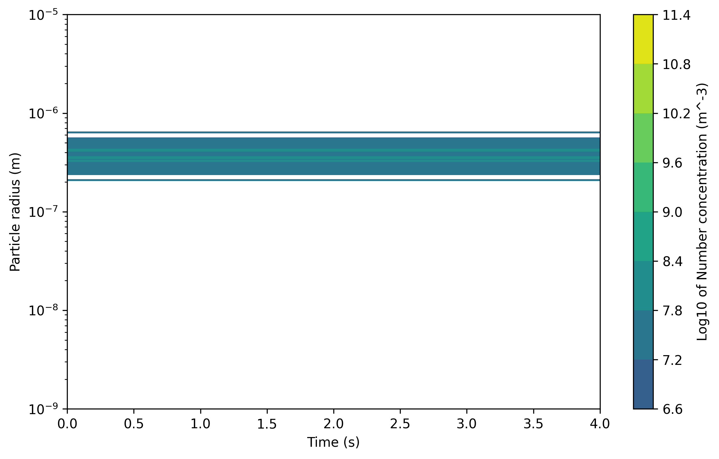
Python · section 9
# plot the total mass and water saturation on twin y-axisfig, ax1 = plt.subplots(figsize=(8, 5))
ax1.plot(time, total_mass_resolved, label="Total mass", color="blue")ax1.set_xlabel("Time (s)")ax1.set_ylabel("Total Particle mass (kg/m^3)", color="blue")ax1.tick_params(axis="y", labelcolor="blue")
ax2 = ax1.twinx()ax2.plot(time, saturation_ratio_output, label="Saturation Ratio", color="red")ax2.set_ylabel("Saturation Ratio", color="red")ax2.tick_params(axis="y", labelcolor="red")
fig.tight_layout()plt.show(block=False)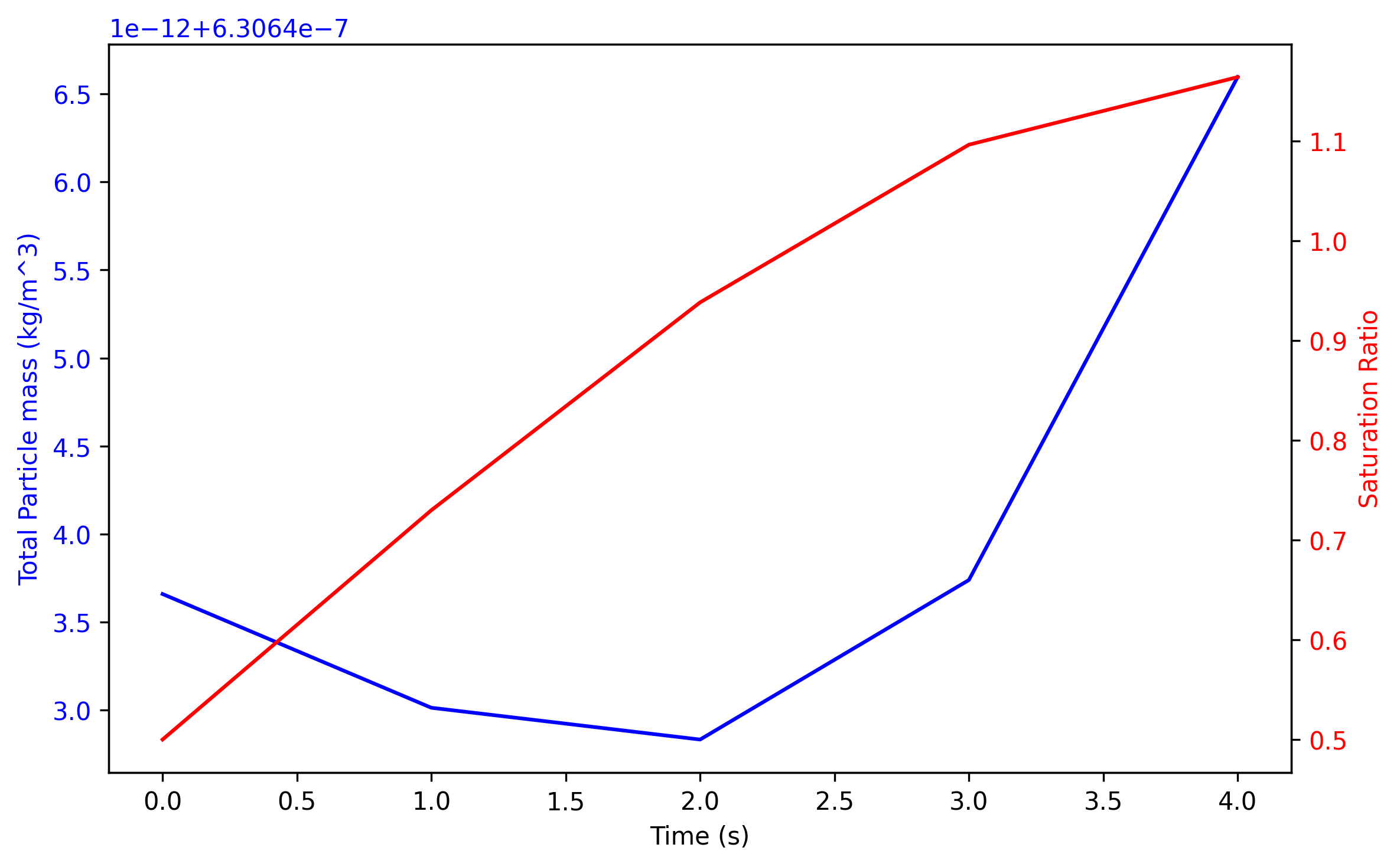
Ask when formation competes with growth
Section titled “Ask when formation competes with growth”This workflow demonstrates how a custom source can be coupled to other processes without losing track of supplied material. Its short trajectory and illustrative rate law do not predict a physical nucleation threshold or atmospheric event.
A useful extension is to vary seed abundance at fixed vapor supply and compare the first nonzero nucleus count, peak saturation, and material partitioning. Repeat with smaller timesteps and alternate process ordering to test whether an apparent threshold is numerical. For production work, use a sourced formation law, explicit applicability limits, and the supported bounded nucleation interface; check slot exhaustion before raising the source strength.
Explore this topic: Nucleation and particle sources