

Compare chamber geometry and competing particle processes
Compare chamber geometry and competing particle processes
Section titled “Compare chamber geometry and competing particle processes”Does a change in particle lifetime come from chamber geometry, or from a process that changes the particles before they reach a wall? This example progresses from wall loss alone to coagulation plus wall loss, then a separate growth-and-loss calculation. It teaches how to read those comparisons without treating every curve as a controlled test of the same factor.
Match the population before changing a mechanism
Section titled “Match the population before changing a mechanism”The shared setup uses 150 radius nodes over 10 nm–10 µm, lognormal radius scales 100 nm and 1 µm, geometric standard deviations 1.2 and 1.4, and modal abundances 10¹⁰ and 10⁹ m⁻³. Density is 1000 kg m⁻³ at 298.15 K and 101325 Pa. The broad preset tails are deliberately excluded here; this is a finite-grid calculation, not a grid-convergence result.
build_aerosol makes a fresh state for each case. run_wall_loss records 61
snapshots over 30 minutes. safe_substeps bounds the explicit loss update using
current sizes, while plot_decay normalizes total number by its initial value.
That positivity bound is not an error estimate for the full coupled sequence.
Python · section 1
import numpy as npimport particula as parfrom matplotlib import pyplot as pltfrom particula.dynamics.condensation.species_mapping import (    CondensationSpeciesMap,)
np.set_printoptions(precision=3, suppress=True)TIME_STEP = 30.0  # secondsTOTAL_TIME = 1800.0  # seconds (30 minutes)N_STEPS = int(TOTAL_TIME / TIME_STEP)TIME_GRID = np.linspace(0.0, TOTAL_TIME, N_STEPS + 1)TEMPERATURE = 298.15  # KPRESSURE = 101325.0  # Pa
Python · section 2
def build_aerosol() -> par.Aerosol:    """Create native bins spanning the two modes with zero initial gas.
    This composition example uses 10 nm–10 µm rather than the preset's    1 nm–100 µm grid: negligible tails on the wider grid can make the    interpolated coagulation rate negative at depleted bins. Native    admission rejects that state; this example does not clamp it away.    """    particles = par.particles.create_lognormal_binned_particle_data(        distribution_type="discrete", radius_bins=np.logspace(-8, -5, 150)    )    gas = par.gas.GasData(        name=["PlaceholderPartitioning", "PlaceholderGasOnly"],        molar_mass=np.array([0.018, 0.028]),        partitioning=np.array([True, False]),        concentration=np.zeros((1, 2)),    )    environment = par.gas.EnvironmentData(        temperature=np.array([TEMPERATURE]),        pressure=np.array([PRESSURE]),        saturation_ratio=np.zeros((1, 2)),    )    return par.Aerosol(particles=particles, gas=gas, environment=environment)

def safe_substeps(strategy, aerosol, duration):    """Bound explicit Euler loss for the current particle sizes."""    coefficient = strategy.loss_coefficient(        aerosol.particles, temperature=TEMPERATURE, pressure=PRESSURE    )    return max(1, int(np.ceil(np.max(coefficient) * duration / 0.9)))

def run_wall_loss(strategy: par.dynamics.WallLossStrategy, sub_steps: int = 1):    """Execute wall loss over the shared time grid."""    aerosol = build_aerosol()    sub_steps = max(sub_steps, safe_substeps(strategy, aerosol, TIME_STEP))    wall_loss = par.dynamics.WallLoss(wall_loss_strategy=strategy)    series = np.zeros_like(TIME_GRID)    series[0] = aerosol.particles.number_density[0]    for idx in range(1, TIME_GRID.size):        aerosol = wall_loss.execute(            aerosol, time_step=TIME_STEP, sub_steps=sub_steps        )        series[idx] = aerosol.particles.number_density[0]    return series, aerosol

def plot_decay(times_min, *series_with_labels):    fig, ax = plt.subplots(figsize=(6, 4))    for series, label, style in series_with_labels:        ax.plot(times_min, series / series[0], style, label=label, linewidth=2)    ax.set_xlabel("Time (min)")    ax.set_ylabel("Normalized concentration")    ax.set_yscale("log")    ax.grid(True)    ax.legend()    plt.tight_layout()    return fig, ax

times_minutes = TIME_GRID / 60.0baseline_aerosol = build_aerosol()print("Initial bins:", baseline_aerosol.particles.radii[0].size)print(    "Initial total conc (1/m^3):",    f"{baseline_aerosol.particles.number_density[0]:.3e}",)
Initial bins: 150
Initial total conc (1/m^3): 1.100e+10Establish the spherical baseline
Section titled “Establish the spherical baseline”The chamber radius is 0.5 m and wall eddy parameter 10⁻³ s⁻¹. The requested two substeps per 30 s interval are increased if the loss coefficient requires more. The saved endpoint is 1.061×10¹⁰ m⁻³ from 1.100×10¹⁰ m⁻³. The first curve shows fractional number remaining; no particle growth or collision process is active.
Python · section 3
spherical_strategy = par.dynamics.SphericalWallLossStrategy( wall_eddy_diffusivity=1e-3, chamber_radius=0.5, distribution_type="discrete",)spherical_series, spherical_aerosol = run_wall_loss( spherical_strategy, sub_steps=2)print("Final conc (spherical):", f"{spherical_series[-1]:.3e} 1/m^3")Final conc (spherical): 1.061e+10 1/m^3Python · section 4
_ = plot_decay( times_minutes, (spherical_series, "Spherical (0.5 m)", "b-"),)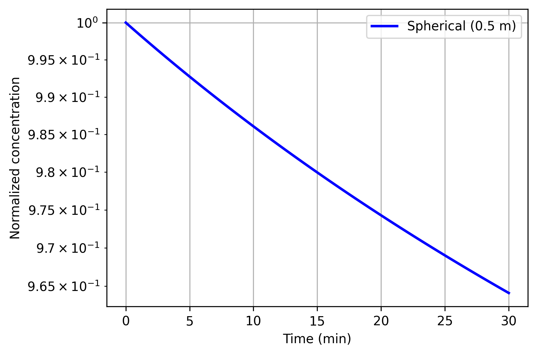
Compare nearly equal chamber volumes
Section titled “Compare nearly equal chamber volumes”The 0.5 m radius sphere has volume about 0.5236 m³; the 1.0 × 0.72 × 0.72 m rectangle has volume 0.5184 m³. They are close, not exactly equal. The initial population and wall eddy parameter match, so the overlay illustrates the geometry dependence of these models with that small volume difference retained. It does not isolate surface area, orientation, or model-form uncertainty.
Python · section 5
rectangular_strategy = par.dynamics.RectangularWallLossStrategy( wall_eddy_diffusivity=1e-3, chamber_dimensions=(1.0, 0.72, 0.72), distribution_type="discrete",)rect_series, _ = run_wall_loss(rectangular_strategy)fig_cmp, _ = plot_decay( times_minutes, (spherical_series, "Spherical (0.5 m)", "b-"), (rect_series, "Rectangular (1.0x0.72x0.72 m)", "r--"),)fig_cmp.axes[0].set_title("Geometry comparison")Text(0.5, 1.0, 'Geometry comparison')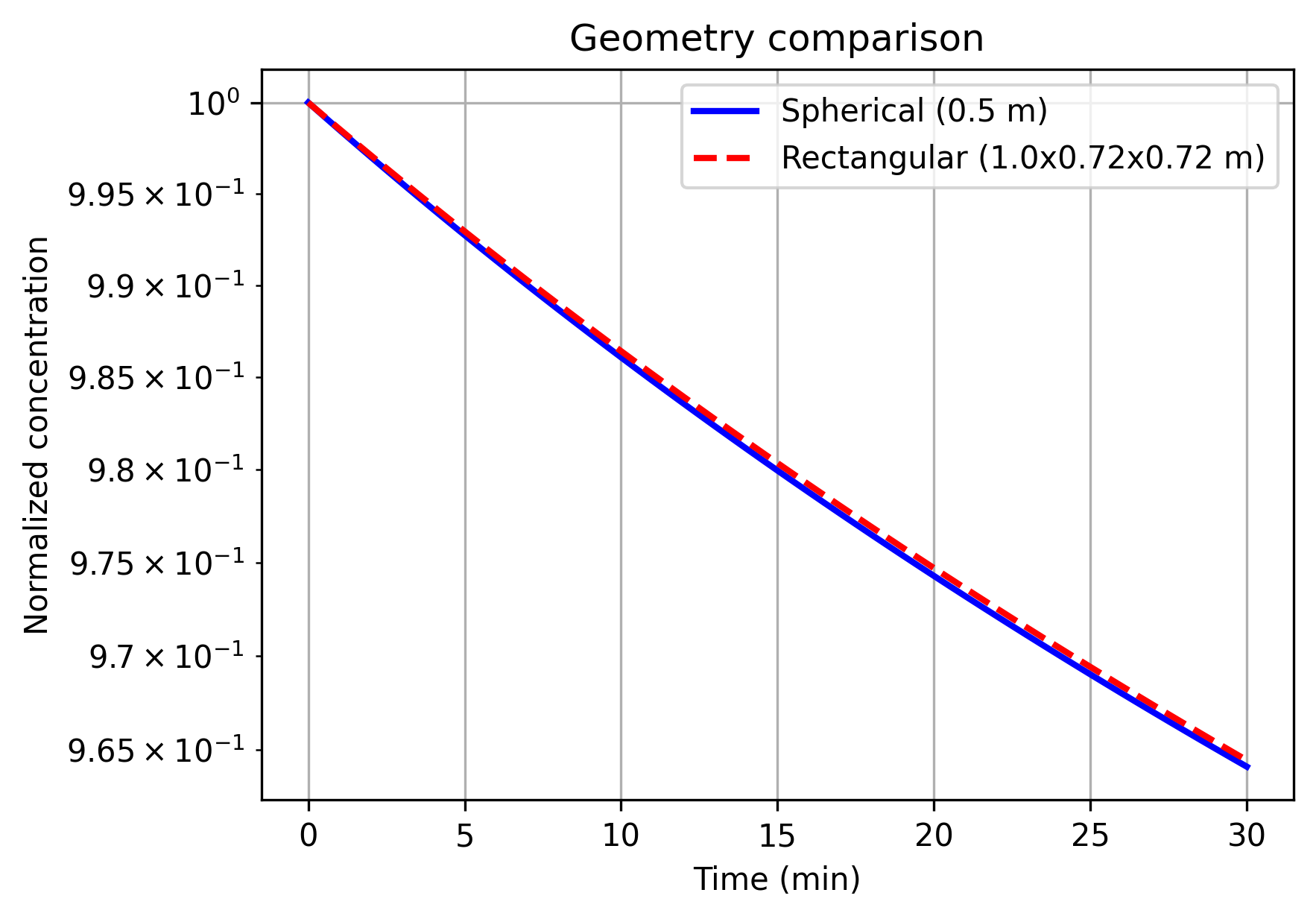
Add collisions to an otherwise matched loss calculation
Section titled “Add collisions to an otherwise matched loss calculation”Fresh populations are advanced with wall loss alone and with Brownian coagulation followed by wall loss. Coagulation changes number and redistributes sizes; wall loss then acts on that evolving spectrum. Compare the two curves to see the combined effect, but do not interpret their difference as the count of particles that coagulated: changing size also changes subsequent wall removal.
The sequence uses | composition and a shared physical interval. Grid refinement,
process ordering, and substep sensitivity are not tested by this overlay.
Python · section 6
coag_strategy = par.dynamics.BrownianCoagulationStrategy(    distribution_type="discrete")coagulation = par.dynamics.Coagulation(coagulation_strategy=coag_strategy)coag_wall = coagulation | par.dynamics.WallLoss(    wall_loss_strategy=spherical_strategy)
aerosol_wall_only = build_aerosol()aerosol_coag_wall = build_aerosol()wall_only_series = np.zeros_like(TIME_GRID)coag_wall_series = np.zeros_like(TIME_GRID)wall_only_series[0] = aerosol_wall_only.particles.number_density[0]coag_wall_series[0] = aerosol_coag_wall.particles.number_density[0]
for idx in range(1, TIME_GRID.size):    aerosol_wall_only = par.dynamics.WallLoss(        wall_loss_strategy=spherical_strategy    ).execute(        aerosol_wall_only,        time_step=TIME_STEP,        sub_steps=safe_substeps(            spherical_strategy, aerosol_wall_only, TIME_STEP        ),    )    aerosol_coag_wall = coag_wall.execute(        aerosol_coag_wall,        time_step=TIME_STEP,        sub_steps=safe_substeps(            spherical_strategy, aerosol_coag_wall, TIME_STEP        ),    )    wall_only_series[idx] = aerosol_wall_only.particles.number_density[0]    coag_wall_series[idx] = aerosol_coag_wall.particles.number_density[0]
_ = plot_decay(    times_minutes,    (wall_only_series, "Wall loss only", "b-"),    (coag_wall_series, "Coagulation | Wall loss", "g--"),)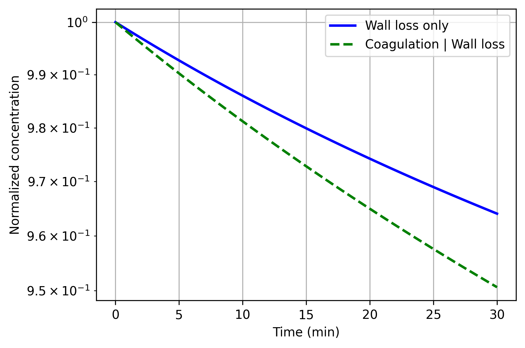
Execution progress
Executing Runnable:   0%|          | 0/1 [00:00<?, ?it/s]
Executing Runnable: 100%|██████████| 1/1 [00:00<00:00, 159.20it/s]
Executing Runnable:   0%|          | 0/1 [00:00<?, ?it/s]
Executing Runnable: 100%|██████████| 1/1 [00:00<00:00, 170.65it/s]
Executing Runnable:   0%|          | 0/1 [00:00<?, ?it/s]
Executing Runnable: 100%|██████████| 1/1 [00:00<00:00, 171.88it/s]
Executing Runnable:   0%|          | 0/1 [00:00<?, ?it/s]
Executing Runnable: 100%|██████████| 1/1 [00:00<00:00, 168.82it/s]
Executing Runnable:   0%|          | 0/1 [00:00<?, ?it/s]
Executing Runnable: 100%|██████████| 1/1 [00:00<00:00, 154.52it/s]
Executing Runnable:   0%|          | 0/1 [00:00<?, ?it/s]
Executing Runnable: 100%|██████████| 1/1 [00:00<00:00, 166.84it/s]
Executing Runnable:   0%|          | 0/1 [00:00<?, ?it/s]
Executing Runnable: 100%|██████████| 1/1 [00:00<00:00, 165.92it/s]
Executing Runnable:   0%|          | 0/1 [00:00<?, ?it/s]
Executing Runnable: 100%|██████████| 1/1 [00:00<00:00, 171.15it/s]
Executing Runnable:   0%|          | 0/1 [00:00<?, ?it/s]
Executing Runnable: 100%|██████████| 1/1 [00:00<00:00, 170.52it/s]
Executing Runnable:   0%|          | 0/1 [00:00<?, ?it/s]
Executing Runnable: 100%|██████████| 1/1 [00:00<00:00, 172.99it/s]
Executing Runnable:   0%|          | 0/1 [00:00<?, ?it/s]
Executing Runnable: 100%|██████████| 1/1 [00:00<00:00, 167.15it/s]
Executing Runnable:   0%|          | 0/1 [00:00<?, ?it/s]
Executing Runnable: 100%|██████████| 1/1 [00:00<00:00, 168.58it/s]
Executing Runnable:   0%|          | 0/1 [00:00<?, ?it/s]
Executing Runnable: 100%|██████████| 1/1 [00:00<00:00, 156.55it/s]
Executing Runnable:   0%|          | 0/1 [00:00<?, ?it/s]
Executing Runnable: 100%|██████████| 1/1 [00:00<00:00, 156.76it/s]
Executing Runnable:   0%|          | 0/1 [00:00<?, ?it/s]
Executing Runnable: 100%|██████████| 1/1 [00:00<00:00, 162.16it/s]
Executing Runnable:   0%|          | 0/1 [00:00<?, ?it/s]
Executing Runnable: 100%|██████████| 1/1 [00:00<00:00, 153.74it/s]
Executing Runnable:   0%|          | 0/1 [00:00<?, ?it/s]
Executing Runnable: 100%|██████████| 1/1 [00:00<00:00, 167.57it/s]
Executing Runnable:   0%|          | 0/1 [00:00<?, ?it/s]
Executing Runnable: 100%|██████████| 1/1 [00:00<00:00, 169.15it/s]
Executing Runnable:   0%|          | 0/1 [00:00<?, ?it/s]
Executing Runnable: 100%|██████████| 1/1 [00:00<00:00, 174.28it/s]
Executing Runnable:   0%|          | 0/1 [00:00<?, ?it/s]
Executing Runnable: 100%|██████████| 1/1 [00:00<00:00, 155.51it/s]
Executing Runnable:   0%|          | 0/1 [00:00<?, ?it/s]
Executing Runnable: 100%|██████████| 1/1 [00:00<00:00, 163.60it/s]
Executing Runnable:   0%|          | 0/1 [00:00<?, ?it/s]
Executing Runnable: 100%|██████████| 1/1 [00:00<00:00, 147.37it/s]
Executing Runnable:   0%|          | 0/1 [00:00<?, ?it/s]
Executing Runnable: 100%|██████████| 1/1 [00:00<00:00, 164.96it/s]
Executing Runnable:   0%|          | 0/1 [00:00<?, ?it/s]
Executing Runnable: 100%|██████████| 1/1 [00:00<00:00, 167.25it/s]
Executing Runnable:   0%|          | 0/1 [00:00<?, ?it/s]
Executing Runnable: 100%|██████████| 1/1 [00:00<00:00, 171.55it/s]
Executing Runnable:   0%|          | 0/1 [00:00<?, ?it/s]
Executing Runnable: 100%|██████████| 1/1 [00:00<00:00, 170.74it/s]
Executing Runnable:   0%|          | 0/1 [00:00<?, ?it/s]
Executing Runnable: 100%|██████████| 1/1 [00:00<00:00, 165.23it/s]
Executing Runnable:   0%|          | 0/1 [00:00<?, ?it/s]
Executing Runnable: 100%|██████████| 1/1 [00:00<00:00, 156.98it/s]
Executing Runnable:   0%|          | 0/1 [00:00<?, ?it/s]
Executing Runnable: 100%|██████████| 1/1 [00:00<00:00, 165.41it/s]
Executing Runnable:   0%|          | 0/1 [00:00<?, ?it/s]
Executing Runnable: 100%|██████████| 1/1 [00:00<00:00, 164.84it/s]
Executing Runnable:   0%|          | 0/1 [00:00<?, ?it/s]
Executing Runnable: 100%|██████████| 1/1 [00:00<00:00, 168.60it/s]
Executing Runnable:   0%|          | 0/1 [00:00<?, ?it/s]
Executing Runnable: 100%|██████████| 1/1 [00:00<00:00, 170.97it/s]
Executing Runnable:   0%|          | 0/1 [00:00<?, ?it/s]
Executing Runnable: 100%|██████████| 1/1 [00:00<00:00, 169.85it/s]
Executing Runnable:   0%|          | 0/1 [00:00<?, ?it/s]
Executing Runnable: 100%|██████████| 1/1 [00:00<00:00, 168.62it/s]
Executing Runnable:   0%|          | 0/1 [00:00<?, ?it/s]
Executing Runnable: 100%|██████████| 1/1 [00:00<00:00, 168.28it/s]
Executing Runnable:   0%|          | 0/1 [00:00<?, ?it/s]
Executing Runnable: 100%|██████████| 1/1 [00:00<00:00, 165.12it/s]
Executing Runnable:   0%|          | 0/1 [00:00<?, ?it/s]
Executing Runnable: 100%|██████████| 1/1 [00:00<00:00, 164.86it/s]
Executing Runnable:   0%|          | 0/1 [00:00<?, ?it/s]
Executing Runnable: 100%|██████████| 1/1 [00:00<00:00, 166.08it/s]
Executing Runnable:   0%|          | 0/1 [00:00<?, ?it/s]
Executing Runnable: 100%|██████████| 1/1 [00:00<00:00, 177.25it/s]
Executing Runnable:   0%|          | 0/1 [00:00<?, ?it/s]
Executing Runnable: 100%|██████████| 1/1 [00:00<00:00, 174.46it/s]
Executing Runnable:   0%|          | 0/1 [00:00<?, ?it/s]
Executing Runnable: 100%|██████████| 1/1 [00:00<00:00, 159.00it/s]
Executing Runnable:   0%|          | 0/1 [00:00<?, ?it/s]
Executing Runnable: 100%|██████████| 1/1 [00:00<00:00, 161.41it/s]
Executing Runnable:   0%|          | 0/1 [00:00<?, ?it/s]
Executing Runnable: 100%|██████████| 1/1 [00:00<00:00, 163.37it/s]
Executing Runnable:   0%|          | 0/1 [00:00<?, ?it/s]
Executing Runnable: 100%|██████████| 1/1 [00:00<00:00, 154.58it/s]
Executing Runnable:   0%|          | 0/1 [00:00<?, ?it/s]
Executing Runnable: 100%|██████████| 1/1 [00:00<00:00, 161.97it/s]
Executing Runnable:   0%|          | 0/1 [00:00<?, ?it/s]
Executing Runnable: 100%|██████████| 1/1 [00:00<00:00, 165.08it/s]
Executing Runnable:   0%|          | 0/1 [00:00<?, ?it/s]
Executing Runnable: 100%|██████████| 1/1 [00:00<00:00, 160.41it/s]
Executing Runnable:   0%|          | 0/1 [00:00<?, ?it/s]
Executing Runnable: 100%|██████████| 1/1 [00:00<00:00, 165.48it/s]
Executing Runnable:   0%|          | 0/1 [00:00<?, ?it/s]
Executing Runnable: 100%|██████████| 1/1 [00:00<00:00, 160.46it/s]
Executing Runnable:   0%|          | 0/1 [00:00<?, ?it/s]
Executing Runnable: 100%|██████████| 1/1 [00:00<00:00, 144.65it/s]
Executing Runnable:   0%|          | 0/1 [00:00<?, ?it/s]
Executing Runnable: 100%|██████████| 1/1 [00:00<00:00, 149.40it/s]
Executing Runnable:   0%|          | 0/1 [00:00<?, ?it/s]
Executing Runnable: 100%|██████████| 1/1 [00:00<00:00, 158.69it/s]
Executing Runnable:   0%|          | 0/1 [00:00<?, ?it/s]
Executing Runnable: 100%|██████████| 1/1 [00:00<00:00, 159.75it/s]
Executing Runnable:   0%|          | 0/1 [00:00<?, ?it/s]
Executing Runnable: 100%|██████████| 1/1 [00:00<00:00, 164.26it/s]
Executing Runnable:   0%|          | 0/1 [00:00<?, ?it/s]
Executing Runnable: 100%|██████████| 1/1 [00:00<00:00, 161.15it/s]
Executing Runnable:   0%|          | 0/1 [00:00<?, ?it/s]
Executing Runnable: 100%|██████████| 1/1 [00:00<00:00, 167.40it/s]
Executing Runnable:   0%|          | 0/1 [00:00<?, ?it/s]
Executing Runnable: 100%|██████████| 1/1 [00:00<00:00, 158.81it/s]
Executing Runnable:   0%|          | 0/1 [00:00<?, ?it/s]
Executing Runnable: 100%|██████████| 1/1 [00:00<00:00, 164.09it/s]
Executing Runnable:   0%|          | 0/1 [00:00<?, ?it/s]
Executing Runnable: 100%|██████████| 1/1 [00:00<00:00, 166.60it/s]
Executing Runnable:   0%|          | 0/1 [00:00<?, ?it/s]
Executing Runnable: 100%|██████████| 1/1 [00:00<00:00, 161.16it/s]
Keep the growth example’s reservoir assumption visible
Section titled “Keep the growth example’s reservoir assumption visible”This separate ten-minute case uses a maintained illustrative organic gas
concentration of 10⁻⁸ kg m⁻³, constant vapor pressure 10⁻⁵ Pa, and molar mass
0.12 kg mol⁻¹ for the mapped species. These are demonstration properties,
not a calibrated organic compound. update_gases=False means particle uptake
is supplied by an external reservoir.
Condensation is applied before spherical wall loss. The plotted diagnostic is total particle number, so it does not directly measure condensed mass. This panel has a different duration and gas setup from the earlier comparisons; it does not establish how much growth alone changes lifetime.
Python · section 7
short_time = np.linspace(0.0, 600.0, 21) # 10 min, 30 s spacingcond_series = np.zeros_like(short_time)# The former zero-gas/high-volatility placeholder could fully evaporate bins# and was silently skipped on failure. Use an explicitly illustrative low-# volatility organic reservoir for this runnable composition demonstration.aerosol_cond = build_aerosol()aerosol_cond.gas.name[0] = "illustrative-organic"aerosol_cond.gas.molar_mass[0] = 0.12aerosol_cond.gas.concentration[0, 0] = 1e-8condensation_strategy = par.dynamics.CondensationIsothermal( molar_mass=aerosol_cond.gas.molar_mass.copy(), diffusion_coefficient=1e-5, accommodation_coefficient=0.9, update_gases=False, activity_strategy=par.particles.ActivityIdealMass(), surface_strategy=par.particles.SurfaceStrategyVolume( surface_tension=0.072, density=1000.0, ), vapor_pressure_strategy=[ par.gas.ConstantVaporPressureStrategy(1e-5), par.gas.ConstantVaporPressureStrategy(1e3), ], species_map=CondensationSpeciesMap(tuple(aerosol_cond.gas.name), ((0, 0),)),)condensation = par.dynamics.MassCondensation(condensation_strategy)wall_loss_runnable = par.dynamics.WallLoss(spherical_strategy)cond_wall = condensation | wall_loss_runnablecond_series[0] = aerosol_cond.particles.number_density[0]for idx in range(1, short_time.size): aerosol_cond = cond_wall.execute( aerosol_cond, time_step=short_time[1] - short_time[0], sub_steps=safe_substeps(spherical_strategy, aerosol_cond, TIME_STEP), ) cond_series[idx] = aerosol_cond.particles.number_density[0]assert np.all(np.isfinite(cond_series))assert np.all(np.diff(cond_series) <= 0)_ = plot_decay( short_time / 60.0, (cond_series, "Condensation | Wall loss (10 min)", "m-"),)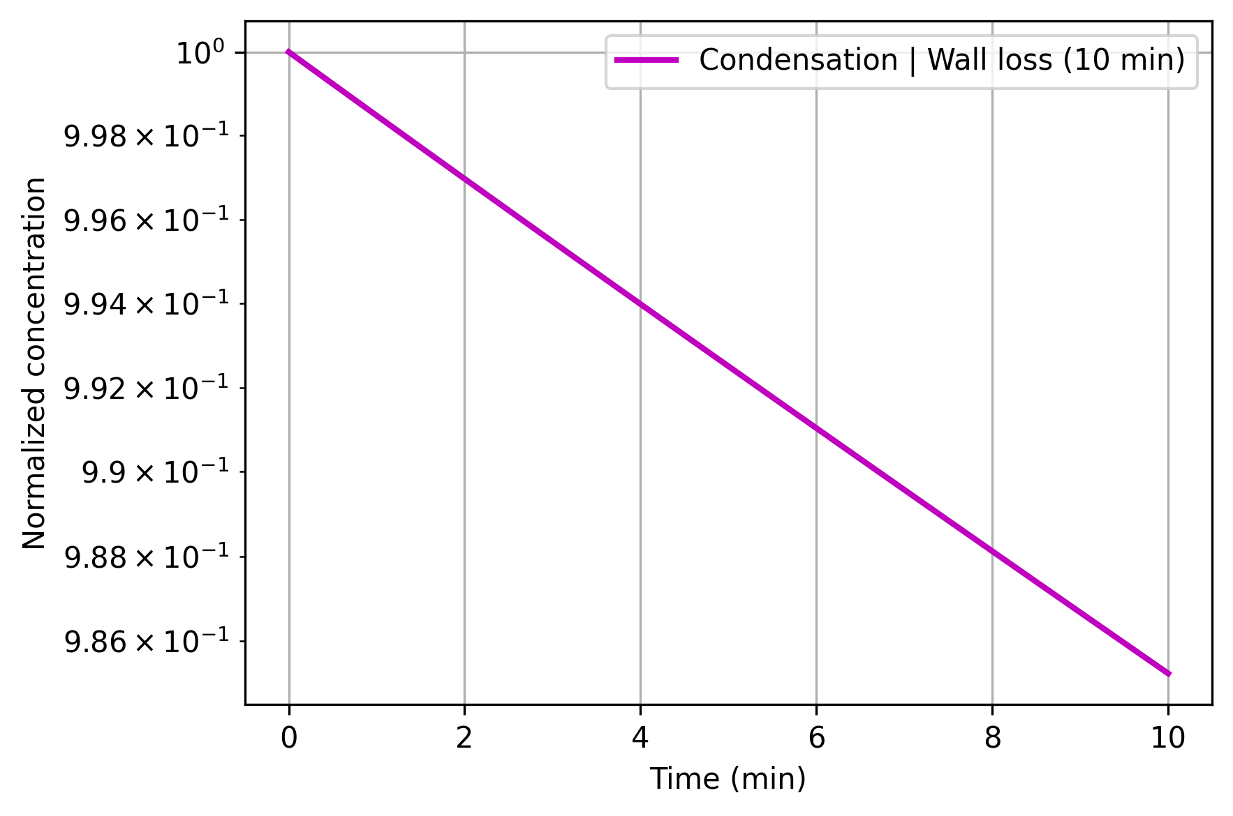
Execution progress
Executing Runnable:   0%|          | 0/1 [00:00<?, ?it/s]
Executing Runnable: 100%|██████████| 1/1 [00:00<00:00, 390.46it/s]
Executing Runnable:   0%|          | 0/1 [00:00<?, ?it/s]
Executing Runnable: 100%|██████████| 1/1 [00:00<00:00, 458.34it/s]
Executing Runnable:   0%|          | 0/1 [00:00<?, ?it/s]
Executing Runnable: 100%|██████████| 1/1 [00:00<00:00, 408.05it/s]
Executing Runnable:   0%|          | 0/1 [00:00<?, ?it/s]
Executing Runnable: 100%|██████████| 1/1 [00:00<00:00, 488.56it/s]
Executing Runnable:   0%|          | 0/1 [00:00<?, ?it/s]
Executing Runnable: 100%|██████████| 1/1 [00:00<00:00, 483.55it/s]
Executing Runnable:   0%|          | 0/1 [00:00<?, ?it/s]
Executing Runnable: 100%|██████████| 1/1 [00:00<00:00, 481.16it/s]
Executing Runnable:   0%|          | 0/1 [00:00<?, ?it/s]
Executing Runnable: 100%|██████████| 1/1 [00:00<00:00, 507.23it/s]
Executing Runnable:   0%|          | 0/1 [00:00<?, ?it/s]
Executing Runnable: 100%|██████████| 1/1 [00:00<00:00, 473.29it/s]
Executing Runnable:   0%|          | 0/1 [00:00<?, ?it/s]
Executing Runnable: 100%|██████████| 1/1 [00:00<00:00, 419.68it/s]
Executing Runnable:   0%|          | 0/1 [00:00<?, ?it/s]
Executing Runnable: 100%|██████████| 1/1 [00:00<00:00, 521.16it/s]
Executing Runnable:   0%|          | 0/1 [00:00<?, ?it/s]
Executing Runnable: 100%|██████████| 1/1 [00:00<00:00, 492.64it/s]
Executing Runnable:   0%|          | 0/1 [00:00<?, ?it/s]
Executing Runnable: 100%|██████████| 1/1 [00:00<00:00, 478.53it/s]
Executing Runnable:   0%|          | 0/1 [00:00<?, ?it/s]
Executing Runnable: 100%|██████████| 1/1 [00:00<00:00, 512.56it/s]
Executing Runnable:   0%|          | 0/1 [00:00<?, ?it/s]
Executing Runnable: 100%|██████████| 1/1 [00:00<00:00, 517.88it/s]
Executing Runnable:   0%|          | 0/1 [00:00<?, ?it/s]
Executing Runnable: 100%|██████████| 1/1 [00:00<00:00, 525.01it/s]
Executing Runnable:   0%|          | 0/1 [00:00<?, ?it/s]
Executing Runnable: 100%|██████████| 1/1 [00:00<00:00, 520.39it/s]
Executing Runnable:   0%|          | 0/1 [00:00<?, ?it/s]
Executing Runnable: 100%|██████████| 1/1 [00:00<00:00, 524.29it/s]
Executing Runnable:   0%|          | 0/1 [00:00<?, ?it/s]
Executing Runnable: 100%|██████████| 1/1 [00:00<00:00, 460.56it/s]
Executing Runnable:   0%|          | 0/1 [00:00<?, ?it/s]
Executing Runnable: 100%|██████████| 1/1 [00:00<00:00, 350.69it/s]
Executing Runnable:   0%|          | 0/1 [00:00<?, ?it/s]
Executing Runnable: 100%|██████████| 1/1 [00:00<00:00, 438.41it/s]
Check valid inputs and admissible output
Section titled “Check valid inputs and admissible output”The final checks reject invalid chamber dimensions and require nonnegative number histories. They do not test closed-system mass conservation, which would be inappropriate for deposition and the maintained vapor reservoir, nor do they establish numerical convergence.
Python · section 8
# Geometry parameter validationtry:    par.dynamics.SphericalWallLossStrategy(        wall_eddy_diffusivity=1e-3, chamber_radius=-1.0    )    raise AssertionError("Expected ValueError for negative radius")except ValueError:    pass
try:    par.dynamics.RectangularWallLossStrategy(        wall_eddy_diffusivity=1e-3, chamber_dimensions=(0.0, 1.0, 1.0)    )    raise AssertionError("Expected ValueError for non-positive dimension")except ValueError:    pass
# Concentration non-negativity after simulationsfor name, series in [    ("spherical", spherical_series),    ("rectangular", rect_series),    ("wall only", wall_only_series),    ("coagulation | wall", coag_wall_series),    ("condensation | wall", cond_series),]:    if not np.all(series >= 0.0):        raise AssertionError(f"Non-negative concentrations failed for {name}")
print("Assertions passed: parameter guards and non-negativity checks.")
Assertions passed: parameter guards and non-negativity checks.Design the next comparison around one question
Section titled “Design the next comparison around one question”These cases show how geometry and coupled dynamics enter a chamber model. To ask whether growth changes deposition significantly, run growth-plus-wall-loss and wall-loss-only cases with identical initial states, gas assumptions, duration, and output diagnostics. Compare size-resolved survival and material removed, then refine timestep and process ordering.
For interpreting an observed decay, use the functional chamber calculation to inspect individual rate contributions. Rate plots can suggest hypotheses; matched process-removal experiments and measurements are needed to test them.
Explore this topic: Wall deposition