

Cooling a gas: saturation without a parcel model
Cooling a gas: saturation without a parcel model
Section titled “Cooling a gas: saturation without a parcel model”Can a fixed amount of vapor become more saturated as its surroundings cool? This diagnostic sweep varies temperature along a prescribed altitude coordinate while holding gas mass concentrations fixed. It connects thermodynamics to gas storage, without simulating transport or condensation.
GasData retains water, butanol, and styrene in one order. EnvironmentData
stores temperature in kelvin, pressure in pascals, and dimensionless saturation
ratios in that gas order. The sweep evaluates only water; zero organic ratios
are unevaluated placeholders, not predictions of organic undersaturation.
Python · section 1
import matplotlib.pyplot as pltimport numpy as npimport particula as parPython · section 2
water_buck = par.gas.VaporPressureFactory().get_strategy("water_buck")butanol_antione = par.gas.VaporPressureFactory().get_strategy( "antoine", {"a": 4.54607 + np.log10(1e5 / 133.322387415), "b": 1351.555, "c": 93.34},)styrene_antione = par.gas.VaporPressureFactory().get_strategy( "antoine", {"a": 4.21948 + np.log10(1e5 / 133.322387415), "b": 1525.059, "c": 56.379},)vapor_pressure_strategies = [water_buck, butanol_antione, styrene_antione]gas_mixture = ( par.gas.GasDataBuilder() .set_names(["water", "butanol", "styrene"]) .set_molar_mass([18.01528e-3, 0.074121, 104.15e-3], "kg/mol") .set_partitioning([True, True, True]) .set_concentration([1e-3, 2e-6, 1e-9], "kg/m^3") .build())environment = par.gas.EnvironmentData( temperature=np.array([298.15]), pressure=np.array([101325.0]), saturation_ratio=np.zeros((1, 3)),)print(gas_mixture)print(environment)GasData(name=['water', 'butanol', 'styrene'], molar_mass=array([0.01801528, 0.074121 , 0.10415 ]), concentration=array([[1.e-03, 2.e-06, 1.e-09]]), partitioning=array([ True, True, True]))
EnvironmentData(temperature=array([298.15]), pressure=array([101325.]), saturation_ratio=array([[0., 0., 0.]]))Prescribe conditions, then evaluate water saturation
Section titled “Prescribe conditions, then evaluate water saturation”The altitude coordinate spans 0–10 km. Temperature follows
Here
At each point, water saturation concentration is recalculated and the fixed 1 g m⁻³ vapor concentration is divided by it. The implementation’s Buck relation switches branches below freezing, so the cold portion uses an ice reference. The recorded total pressure does not enter this particular ratio calculation. Read the plot as a thermodynamic diagnostic under those assumptions.
Python · section 3
# Constants for calculationssea_level_pressure = 101325  # Reference pressure at sea level (Pa)sea_level_temperature = 288.15  # Reference temperature at sea level (K)gravity = 9.80665  # Acceleration due to gravity (m/s^2)molar_mass_air = 0.0289644  # Molar mass of Earth's air (kg/mol)universal_gas_constant = 8.314  # Universal gas constant (J/(mol·K))temperature_lapse_rate = 0.0065  # Standard temperature lapse rate (K/m)
# Generate an array of altitudes from sea level (0 meters) to 10 km (10000 meters), divided into 100 intervalsaltitude_range = np.linspace(0, 10000, 100)
# Calculate the temperature at each altitude based on the linear temperature lapse ratetemperature_at_altitudes = (    sea_level_temperature - temperature_lapse_rate * altitude_range)
# Calculate the pressure at each altitude using the barometric formulapressure_at_altitudes = sea_level_pressure * (    (1 - temperature_lapse_rate * altitude_range / sea_level_temperature)    ** (        gravity        * molar_mass_air        / (universal_gas_constant * temperature_lapse_rate)    ))

# Only water is evaluated over this cold altitude range. The organic Antoine# coefficients are not qualified here; gas storage still retains those lanes.# Saturation-ratio lanes for organics remain their prescribed initial values.saturation_ratio = np.zeros(len(altitude_range))for index, (temperature, pressure) in enumerate(    zip(temperature_at_altitudes, pressure_at_altitudes, strict=True)):    environment.temperature[0] = temperature    environment.pressure[0] = pressure    saturation = water_buck.saturation_concentration(        gas_mixture.molar_mass[0], temperature    )    environment.saturation_ratio[0, 0] = (        gas_mixture.concentration[0, 0] / saturation    )    saturation_ratio[index] = environment.saturation_ratio[0, 0]
# Plot the saturation ratio of water vapor at each altitudefig, ax = plt.subplots()ax.plot(saturation_ratio, altitude_range, label="Water")ax.set_xscale("log")ax.set_ylabel("Altitude (m)")ax.set_xlabel("Water Saturation Ratio")ax.set_title("Saturation Ratio of Water Vapor at Different Altitudes")ax.legend()plt.show()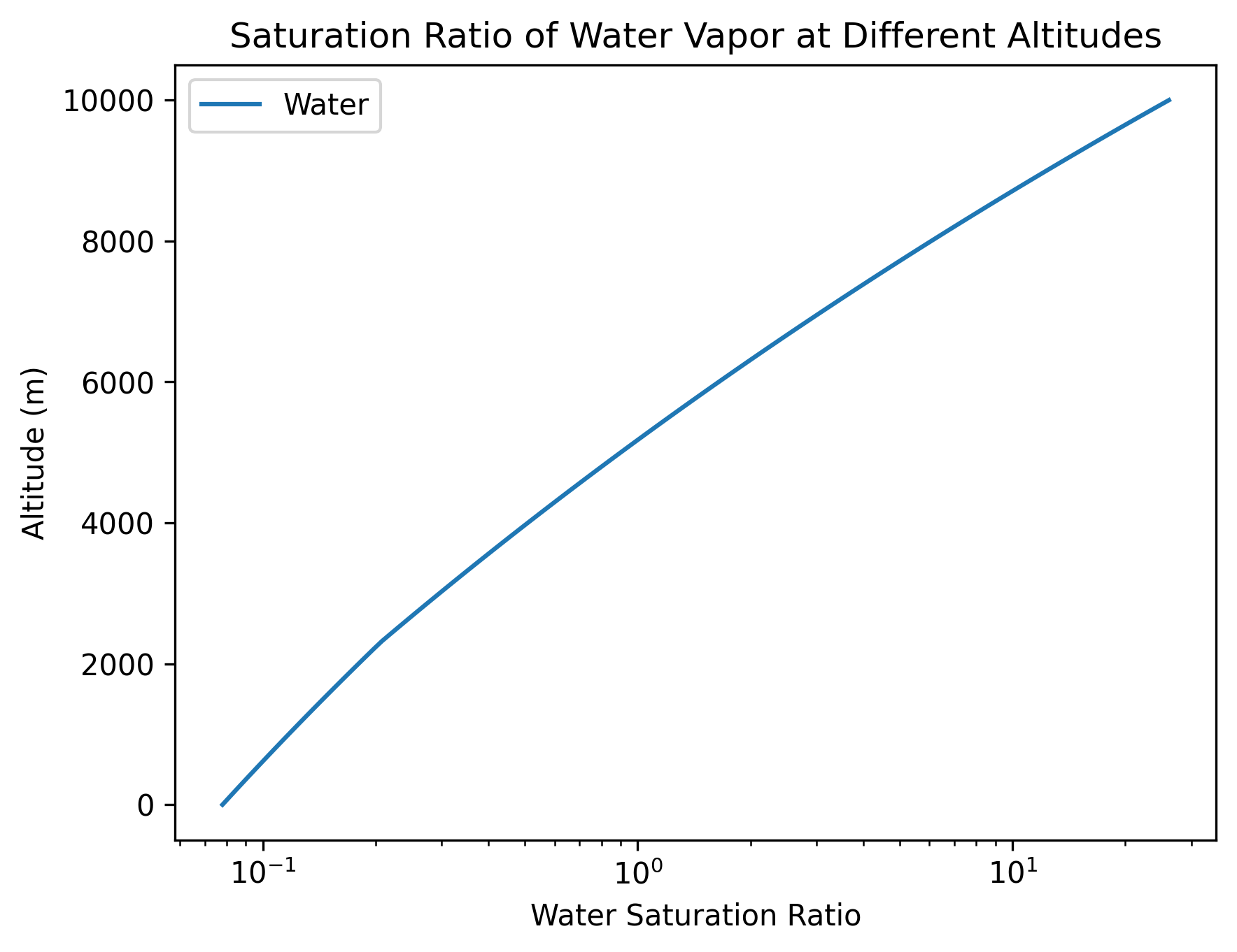
What the curve can tell you
Section titled “What the curve can tell you”The curve shows how the same vapor concentration compares with a changing saturation reference. A ratio above one signals supersaturation relative to that reference; this calculation does not remove excess vapor or predict cloud onset. Particle composition, curvature, and kinetics are not represented.
For a cooling-chamber study, replace the prescribed temperature history with measured conditions, evolve vapor depletion alongside particles, and account for thermal feedback where needed. Compare this fixed-vapor diagnostic with the coupled calculation to separate thermodynamic forcing from vapor consumption. The staggered condensation example is a next step toward that coupled question.
Explore this topic: Gas and environment