

Follow collisions through individual particles
Python · section 1
"""Demonstrate particle-resolved Brownian coagulation.
Generates a modest bimodal particle-resolved sample, configures Browniancoagulation with ``distribution_type="particle_resolved"``, runs a shortstep, and plots histograms of radii before/after execution to show how thesample redistributes. Uses a small sample size to keep runtime fast.
Example:    Run the script to visualize how Brownian coagulation redistributes a    set of sampled radii in a particle-resolved representation via the    public ``par.dynamics`` API."""
'Demonstrate particle-resolved Brownian coagulation.\n\nGenerates a modest bimodal particle-resolved sample, configures Brownian\ncoagulation with ``distribution_type="particle_resolved"``, runs a short\nstep, and plots histograms of radii before/after execution to show how the\nsample redistributes. Uses a small sample size to keep runtime fast.\n\nExample:\n Run the script to visualize how Brownian coagulation redistributes a\n set of sampled radii in a particle-resolved representation via the\n public ``par.dynamics`` API.\n'Follow collisions through individual particles
Section titled “Follow collisions through individual particles”What can an individual-particle representation reveal that a smooth size curve hides? Each active slot carries mass, and a collision changes the surviving particles and their counts. This single-material example establishes the inventory accounting needed before studying composition mixing.
Compare with the bin example, but note that its initial concentration and distribution differ. These two pages demonstrate representations; they are not a controlled accuracy or speed comparison.
Python · section 2
# In Colab uncomment the following command to install particula:# Install from the repository root: `python -m pip install -e ".[extra]"`import matplotlib.pyplot as pltimport numpy as npimport particula as parGive sampled particles a physical volume
Section titled “Give sampled particles a physical volume”The initial sample contains 50,000 radii from two lognormal components with 80 and 200 nm radius scales, geometric standard deviations 1.4 and 1.5, and relative weights 40,000:20,000. Unit represented counts in 10⁻³ m³ give an initial number density of 5×10⁷ m⁻³. Density is 1000 kg m⁻³; the environment stays at 298.15 K and 101325 Pa.
The sampling seed makes this initial population reproducible. It does not supply an uncertainty interval or guarantee identical collision histories across execution backends.
Python · section 3
# Seed the illustrative sampling; this is not cross-backend replay.np.random.seed(42)# Sample radii (published 50,000-particle workload)radii_sample = par.particles.get_lognormal_sample_distribution(    mode=np.array([80e-9, 200e-9]),    geometric_standard_deviation=np.array([1.4, 1.5]),    number_of_particles=np.array([4e4, 2e4]),    number_of_samples=50_000,)
density = np.array([1_000.0])mass_sample = 4 / 3 * np.pi * radii_sample**3 * density
# Native ambient environment. GasData requires a species axis, so a# zero-concentration, non-partitioning carrier fills that axis. Coagulation# does not consume it; ambient pressure is specified independently.environment = par.gas.EnvironmentData(    temperature=np.array([298.15]),    pressure=np.array([101325.0]),    saturation_ratio=np.zeros((1, 1)),)gas = par.gas.GasData(    name=["carrier"],    molar_mass=np.array([0.02897]),    partitioning=np.array([False]),    concentration=np.zeros((1, 1)),)# Unit count weights represent 50,000 particles in 1e-3 m³.particles_resolved = par.particles.create_resolved_particle_data(    masses=mass_sample,    density=density,    volume=1e-3,)aerosol_resolved = par.Aerosol(    particles=particles_resolved,    gas=gas,    environment=environment,)
Choose the collision mechanism
Section titled “Choose the collision mechanism”The particle-resolved Brownian strategy merges sampled particles using the size-dependent kernel. The carrier gas is non-partitioning; this calculation has no condensation or external source. Count and mass diagnostics can therefore be interpreted as collision effects within this closed particle inventory.
Python · section 4
coagulation_strategy = (    par.dynamics.BrownianCoagulationBuilder()    .set_distribution_type("particle_resolved")    .build())coagulation_process = par.dynamics.Coagulation(    coagulation_strategy=coagulation_strategy)
print(coagulation_process)
<particula.dynamics.particle_process.Coagulation object at 0x7f3d60b51430>Advance one hour and check the inventory
Section titled “Advance one hour and check the inventory”The call advances 3600 s with 20 substeps. The assertions require nonnegative counts, no increase in total represented count, and conservation of the count-weighted material inventory within the stated tolerance. Inactive slots are excluded from the final radius sample. Array capacity is not the number of surviving physical particles.
Python · section 5
time_step = 3600  # seconds (1 hour)sub_steps = 20
radii_before = aerosol_resolved.particles.radii[0].copy()initial_mass = np.sum(    aerosol_resolved.particles.masses    * aerosol_resolved.particles.concentration[..., None],    axis=1,)
aerosol_after = coagulation_process.execute(    aerosol_resolved, time_step=time_step, sub_steps=sub_steps)radii_after = aerosol_after.particles.radii[0]np.testing.assert_allclose(    np.sum(        aerosol_after.particles.masses        * aerosol_after.particles.concentration[..., None],        axis=1,    ),    initial_mass,    rtol=1e-12,    atol=1e-30,)assert np.all(aerosol_after.particles.masses >= 0)assert np.sum(aerosol_after.particles.concentration) <= 50_000# Free slots have radius zero; exclude them from the normalized active PDF.radii_after = radii_after[aerosol_after.particles.concentration[0] > 0]
Separate size-distribution shape from number loss
Section titled “Separate size-distribution shape from number loss”Both histograms use density=True: their areas are normalized independently.
They show probability density per metre of radius, not physical number density.
Thus their areas cannot reveal how many particles disappeared. Read the shape
comparison alongside the count and material checks above; a number-per-volume
histogram would be needed to display abundance on the same figure.
Python · section 6
bins = np.logspace(np.log10(radii_before.min()), -5, 80).tolist()
fig, ax = plt.subplots(figsize=(8, 5))ax.hist(    radii_before,    bins=bins,    histtype="step",    color="tab:blue",    label="Before",    density=True,)ax.hist(    radii_after,    bins=bins,    histtype="step",    color="tab:orange",    label="After",    density=True,)ax.set_xscale("log")ax.set_xlim(1e-8, 1e-5)ax.set_xlabel("Particle radius (m)")ax.set_ylabel("Active-particle probability density (m$^{-1}$)")ax.set_title("Particle-resolved coagulation (Brownian)")ax.legend()ax.grid(alpha=0.3)plt.show()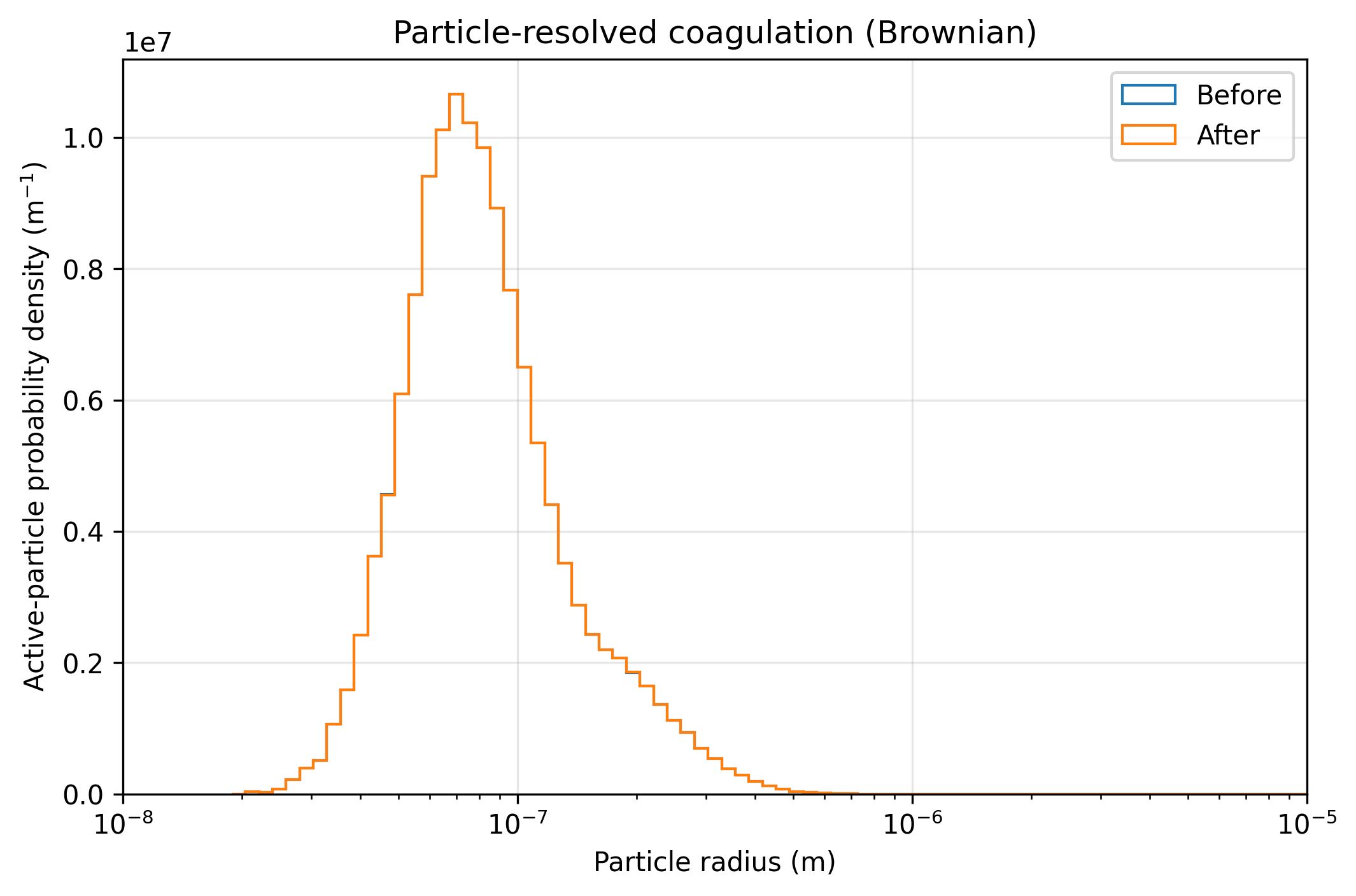
Extend from size to mixing state
Section titled “Extend from size to mixing state”The result demonstrates collision bookkeeping and a change in the sampled size distribution while retaining material. It does not establish convergence from one sample and timestep choice.
A useful next experiment is to initialize two component populations and ask how quickly collisions produce internally mixed particles. Track component-wise inventory, composition conditional on size, and total number; repeat seeds and refine substeps. The time-evolution comparison shows how to match initial physical abundance before comparing representations.
Explore this topic: Particle-resolved populations