

Distinguish dry-phase oscillation from physical droplet relaxation
Distinguish dry-phase oscillation from physical droplet relaxation
Section titled “Distinguish dry-phase oscillation from physical droplet relaxation”Does a wet particle repeatedly grow and shrink after a humidity drop, or is the timestep too large? This controlled calculation compares the existing inventory-limited fixed update with adaptive ROS2/ROS3 and an independent radius equation. A 100 nm dry hygroscopic seed carries water; 10⁸ particles/m³ share a finite vapor reservoir at 298.15 K. At 0.2 s we reset gas water from the wet reservoir to 85% saturation. The reset is an external exchange, not a failure of closed condensation accounting. No collisions or wall loss are included.
This is an illustrative κ=0.5 material, not a chamber fit. Saturation pressure is prescribed as 3168.5 Pa and surface tension as 0.072 N/m. The dry and water densities are both 1000 kg/m³ so the independent radius equation has one unambiguous material density. The full chamber examples retain their distinct material properties and stochastic removal.
Python · section 1
import matplotlib.pyplot as pltimport numpy as npimport particula as parfrom particula.dynamics.condensation.species_mapping import (    CondensationSpeciesMap,)from particula.execution.condensation_ode import CondensationODEfrom scipy.integrate import solve_ivp
R_DRY = 100e-9RHO = 1000.0NUMBER = 1e8TEMPERATURE = 298.15PRESSURE = 101325.0MOLAR = 0.018015DIFFUSION = 2.4e-5KAPPA = 0.5SIGMA = 0.072GAS_CONSTANT = 8.31446261815324C_SAT = 3168.5 * MOLAR / (GAS_CONSTANT * TEMPERATURE)DRY_VOLUME = 4 * np.pi * R_DRY**3 / 3TIMES = np.linspace(0, 0.4, 81)

def build_case():    """Declare native water/dry state and a single volatile material map."""    particles = par.particles.create_resolved_particle_data(        masses=[[RHO * DRY_VOLUME, RHO * DRY_VOLUME]],        density=[RHO, RHO],        concentration=[NUMBER],        volume=1.0,    )    gas = par.gas.GasData(        name=["water"],        molar_mass=np.array([MOLAR]),        concentration=np.array([[1.004 * C_SAT]]),        partitioning=np.array([True]),    )    environment = par.gas.EnvironmentData(        temperature=[TEMPERATURE],        pressure=[PRESSURE],        saturation_ratio=[[0.0]],    )    activity = (        par.particles.ActivityKappaParameterBuilder()        .set_kappa(np.array([KAPPA, 0.0]))        .set_density(np.array([RHO, RHO]), "kg/m^3")        .set_molar_mass(np.array([0.13214, MOLAR]), "kg/mol")        .set_water_index(1)        .build()    )    strategy = par.dynamics.CondensationIsothermal(        molar_mass=np.array([MOLAR]),        diffusion_coefficient=DIFFUSION,        accommodation_coefficient=1.0,        activity_strategy=activity,        surface_strategy=par.particles.SurfaceStrategyVolume(            surface_tension=SIGMA,            density=RHO,        ),        vapor_pressure_strategy=par.gas.ConstantVaporPressureStrategy(3168.5),        species_map=CondensationSpeciesMap(("water",), ((0, 1),)),    )    return par.Aerosol(        particles=particles, gas=gas, environment=environment    ), strategy
Solve an independent water-volume equation
Section titled “Solve an independent water-volume equation”Let x=Vwater/Vdry. Radius is rdry(1+x)^(1/3), water activity is x/(x+κ), and Kelvin curvature multiplies equilibrium vapor by exp(A/r), where A=2σM/(RTρ). Within a closed segment, gas concentration follows its own inventory: C=Cstart−NρVdry(x−xstart). Substituting these into the spherical diffusion flux gives dx/dt=3Dr f(Kn)(C−Ceq)/(ρ rdry³). The kinetic correction uses unit accommodation and the same declared transport law. This reference is written independently of Particula’s mass-transfer and activity functions. Radau and BDF must agree more tightly than the displayed solver error target.
Python · section 2
def reference(method):    """Cross-check a scalar volume equation with two independent SciPy solvers."""    viscosity = (        1.716e-5        * (TEMPERATURE / 273.15) ** 1.5        * 383.55        / (TEMPERATURE + 110.4)    )    mean_free_path = (2 * viscosity / PRESSURE) / np.sqrt(        8 * MOLAR / (np.pi * GAS_CONSTANT * TEMPERATURE)    )    kelvin_length = 2 * SIGMA * MOLAR / (GAS_CONSTANT * TEMPERATURE * RHO)    x = 1.0    water, gas = [], []    for begin, end, concentration in (        (0.0, 0.2, 1.004 * C_SAT),        (0.2, 0.4, 0.85 * C_SAT),    ):        x_start = x        sample = TIMES[(TIMES >= begin) & (TIMES <= end)]
        def rate(time, values, concentration=concentration, x_start=x_start):            volume_ratio = values[0]            radius = R_DRY * np.cbrt(1 + volume_ratio)            kn = mean_free_path / radius            correction = 0.75 * (1 + kn) / (kn**2 + 1.283 * kn + 0.75)            vapor = concentration - NUMBER * RHO * DRY_VOLUME * (                volume_ratio - x_start            )            equilibrium = (                C_SAT                * volume_ratio                / (volume_ratio + KAPPA)                * np.exp(kelvin_length / radius)            )            return [                3                * DIFFUSION                * radius                * correction                * (vapor - equilibrium)                / (RHO * R_DRY**3)            ]
        solved = solve_ivp(            rate,            (begin, end),            [x],            method=method,            t_eval=sample,            rtol=1e-10,            atol=1e-12,            first_step=1e-8,        )        assert solved.success, solved.message        local = solved.y[0]        vapor = concentration - NUMBER * RHO * DRY_VOLUME * (local - x_start)        if water:            water.pop()            gas.pop()  # the event row uses the new gas reservoir        water.extend(local)        gas.extend(vapor)        x = local[-1]    return np.array(water), np.array(gas)

def calculate(method, tolerance=1e-5):    """Observe complete intervals and account separately for the vapor reset."""    state, strategy = build_case()    owner = None    rows, work = [], {"accepted": 0, "rejected": 0, "fixed_steps": 0}    inventory = (        NUMBER * state.particles.masses[0, 0, 1] + state.gas.concentration[0, 0]    )    budget_error = 0.0    for i, time in enumerate(TIMES):        if i:            if method == "fixed":                par.dynamics.MassCondensation(strategy).execute(                    state, time_step=float(time - TIMES[i - 1])                )                work["fixed_steps"] += 1            else:                if owner is None:                    owner = CondensationODE(                        state,                        strategy,                        time=float(TIMES[i - 1]),                        method=method,                        rtol=tolerance,                        particle_atol=1e-27,                        gas_atol=1e-13,                        first_step=1e-6,                        max_step=0.005,                    )                while owner.time < time:                    owner.step(float(time))                state = owner.snapshot()        total = (            NUMBER * state.particles.masses[0, 0, 1]            + state.gas.concentration[0, 0]        )        budget_error = max(budget_error, abs(total - inventory) / inventory)        if time == 0.2:            state.gas.concentration[0, 0] = 0.85 * C_SAT            inventory = (                NUMBER * state.particles.masses[0, 0, 1]                + state.gas.concentration[0, 0]            )            if owner is not None:                work["accepted"] += owner.solver.statistics.accepted                work["rejected"] += owner.solver.statistics.rejected            owner = None        rows.append(            [                state.particles.masses[0, 0, 1] / (RHO * DRY_VOLUME),                state.gas.concentration[0, 0],            ]        )    if owner is not None:        work["accepted"] += owner.solver.statistics.accepted        work["rejected"] += owner.solver.statistics.rejected    assert budget_error < 2e-12    return np.asarray(rows), work, budget_error

def simulate():    """Retain failures of coarse stepping and qualify adaptive observable error."""    reference_water, reference_gas = reference("Radau")    check_water, check_gas = reference("BDF")    np.testing.assert_allclose(        check_water, reference_water, rtol=2e-8, atol=1e-9    )    np.testing.assert_allclose(check_gas, reference_gas, rtol=2e-10, atol=1e-12)    results = {}    for name, method, tolerance in (        ("fixed 0.005 s", "fixed", 1e-5),        ("ROS2 1e-5", "ros2", 1e-5),        ("ROS2 1e-7", "ros2", 1e-7),        ("ROS3 1e-5", "ros3", 1e-5),        ("ROS3 1e-7", "ros3", 1e-7),    ):        values, work, budget = calculate(method, tolerance)        radius = R_DRY * np.cbrt(1 + values[:, 0])        reference_radius = R_DRY * np.cbrt(1 + reference_water)        error = float(np.max(np.abs(radius / reference_radius - 1)))        if tolerance == 1e-7:            assert error < 2e-5, error        results[name] = {            "radius_nm": (radius * 1e9).tolist(),            "gas_kg_m3": values[:, 1].tolist(),            "radius_error": error,            "budget_error": budget,            "work": work,        }    for method in ("ROS2", "ROS3"):        assert (            results[f"{method} 1e-7"]["radius_error"]            < results[f"{method} 1e-5"]["radius_error"]        )    return {        "time_s": TIMES.tolist(),        "reference_radius_nm": (            R_DRY * np.cbrt(1 + reference_water) * 1e9        ).tolist(),        "results": results,        "configuration": {            "dry_radius_m": R_DRY,            "number_m3": NUMBER,            "kappa": KAPPA,        },    }

def plot_results(report):    """Plot saved trajectories and report accuracy separately from mass closure."""    fig, axes = plt.subplots(1, 2, figsize=(11, 4))    axes[0].plot(        report["time_s"],        report["reference_radius_nm"],        color="black",        label="Independent reference",    )    for name, result in report["results"].items():        axes[0].plot(            report["time_s"], result["radius_nm"], label=name, alpha=0.8        )        axes[1].semilogy(            report["time_s"],            np.maximum(                np.abs(                    np.asarray(result["radius_nm"])                    / report["reference_radius_nm"]                    - 1                ),                1e-12,            ),            label=name,        )        print(            name,            "max radius error:",            result["radius_error"],            "mass residual:",            result["budget_error"],            "work:",            result["work"],        )    for axis in axes:        axis.axvline(0.2, color="gray", linestyle=":")        axis.set_xlabel("Time (s)")    axes[0].set_ylabel("Wet radius (nm)")    axes[1].set_ylabel("Relative radius error")    axes[0].legend(fontsize=8)    fig.tight_layout()    plt.show()
Interpret accuracy separately from conservation
Section titled “Interpret accuracy separately from conservation”The printed errors compare the complete trajectory with an independent reference. Tightening either method’s tolerance should reduce radius error; the mass residual tests a different property. A bounded, mass-conserving coarse update may still fail to resolve evaporation. The initial wet growth and dry reset explain why one timestep can behave differently in different parts of a run. In the retained run, the fixed update oscillates after the reset despite a relative mass residual below 10⁻¹⁴. Its maximum relative radius error is about 3.70; ROS2 at tolerances 10⁻⁵ and 10⁻⁷ reduces that error to about 6.05×10⁻⁶ and 6.98×10⁻⁸, respectively. ROS3 achieves about 4.08×10⁻⁶ and 3.39×10⁻⁸ with 330 and 1,247 accepted steps, versus ROS2’s 3,667 and 36,161. Its higher order reduces numerical work in this case; neither order nor conservation guarantees that result in another regime. These are errors for this prescribed case, not universal error bounds for other compositions or cloud histories. For a chamber study, next vary dry composition and outer wall-loss timing while retaining separate source/loss ledgers and convergence checks.
Python · section 3
if __name__ == "__main__": report = simulate() plot_results(report)Explicit cpu invocation
report = simulate()plot_results(report)fixed 0.005 s max radius error: 3.6952062679162676 mass residual: 3.0014944683315325e-16 work: {'accepted': 0, 'rejected': 0, 'fixed_steps': 80}
ROS2 1e-5 max radius error: 6.0462680853135e-06 mass residual: 2.6589178106206993e-15 work: {'accepted': 3667, 'rejected': 2, 'fixed_steps': 0}
ROS2 1e-7 max radius error: 6.984975953194805e-08 mass residual: 1.2408283116111686e-14 work: {'accepted': 36161, 'rejected': 4, 'fixed_steps': 0}
ROS3 1e-5 max radius error: 4.07786147638145e-06 mass residual: 2.481656623139604e-15 work: {'accepted': 330, 'rejected': 0, 'fixed_steps': 0}
ROS3 1e-7 max radius error: 3.390750791254504e-08 mass residual: 2.304395435846458e-15 work: {'accepted': 1247, 'rejected': 2, 'fixed_steps': 0}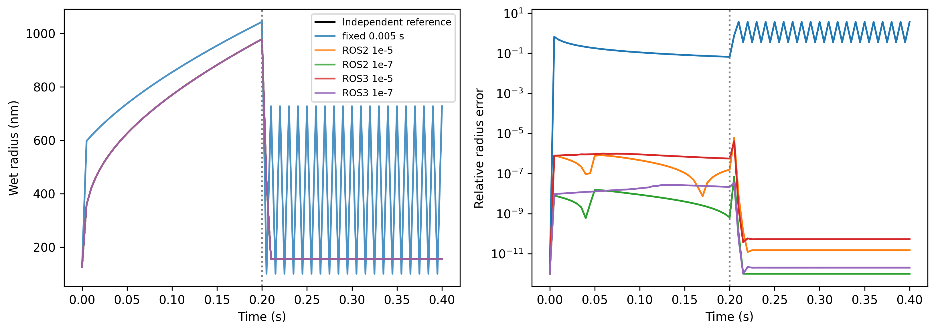
Explore this topic: Adaptive growth and relaxation · Chamber experiments