

Separate size-selective removal from particle growth
Separate size-selective removal from particle growth
Section titled “Separate size-selective removal from particle growth”Can a size distribution change even when no surviving particle changes size? Wall loss removes different radii at different rates. This example follows that effect in a spherical chamber, plotting both total-number decay and the remaining spectrum. The distinction matters when interpreting chamber data that might otherwise be attributed to condensation or coagulation.
Prepare the reference calculation
Section titled “Prepare the reference calculation”Use Python 3.12 or newer, Particula, NumPy, and Matplotlib. Begin with distribution measures if a bin total and a density per radius are unfamiliar. The combined chamber example adds other mechanisms.
Python · section 1
# If running in Colab, uncomment the next line to install particula:# Install from the repository root: `python -m pip install -e ".[extra]"`
import numpy as npimport particula as parfrom matplotlib import pyplot as plt
Specify the initial population
Section titled “Specify the initial population”The preset uses 250 radius nodes from 1 nm–100 µm, lognormal radius scales 100 nm and 1 µm, geometric standard deviations 1.2 and 1.4, and modal number densities 10¹⁰ and 10⁹ m⁻³. Density is 1000 kg m⁻³. These are demonstration inputs, not a chamber measurement. Bin concentrations are in m⁻³ and sum to total number density.
Python · section 2
# Build a simple radius-based particle distribution (discrete bins)particle = par.particles.create_lognormal_binned_particle_data(    distribution_type="discrete")
print("Radius shape:", particle.radii[0].shape)print("Concentration shape:", particle.concentration[0].shape)print(    "Total concentration (initial):",    f"{particle.number_density[0]:.3e} 1/m^3",)
Radius shape: (250,)
Concentration shape: (250,)
Total concentration (initial): 1.100e+10 1/m^3Translate geometry into a loss law
Section titled “Translate geometry into a loss law”The sphere has radius 0.5 m and wall eddy parameter 10⁻³ s⁻¹, at fixed 298.15 K and 101325 Pa. The strategy computes size-dependent first-order loss coefficients. Its rate includes current bin abundance, so the printed first-bin rate is not representative of the entire population.
Python · section 3
# Configure spherical wall loss strategywall_loss = par.dynamics.SphericalWallLossStrategy(    wall_eddy_diffusivity=1e-3,  # 1/s    chamber_radius=0.5,  # m    distribution_type="discrete",)
T = 298.15  # KP = 101325.0  # Pa
rate = wall_loss.rate(    particle=particle,    temperature=T,    pressure=P,)
print("Rate array shape:", rate.shape)print("Example rate[0]:", float(rate.ravel()[0]))
Rate array shape: (250,)
Example rate[0]: -2.2766844125094575e-88Follow 100 minutes, with an explicit discrete reference
Section titled “Follow 100 minutes, with an explicit discrete reference”The run lasts 6000 s (100 minutes) with 1 s output intervals. Internal substeps bound the largest coefficient-times-step product by 0.9; the saved run uses two. This prevents negative concentrations but does not guarantee a desired accuracy.
Fixed radii make repeated Euler decay an independent expression for the expected update. The assertion compares with that expression, checks nonnegative counts, and requires unchanged individual masses. The continuous exponential solution would supply a separate timestep-error comparison.
Python · section 4
# Time integration setupfinal_time = 6000.0  # s (= 100 minutes)dt = 1.0  # sn_steps = int(final_time / dt)
# Native Euler updates reject negative concentrations. Retain the output# interval and full duration, but bound each internal step by max(k) * dt < 1.sub_steps = max(    1,    int(        np.ceil(            np.max(                wall_loss.loss_coefficient(particle, temperature=T, pressure=P)            )            * dt            / 0.9        )    ),)print("Internal substeps per output interval:", sub_steps)times = np.arange(n_steps + 1) * dttotal_concentration = np.zeros_like(times, dtype=float)
initial_counts = particle.concentration.copy()initial_masses = particle.masses.copy()loss_coefficients = wall_loss.loss_coefficient(    particle, temperature=T, pressure=P)# Record initial concentrationtotal_concentration[0] = particle.number_density[0]
# Time loop: apply only wall lossfor i in range(1, n_steps + 1):    for _substep in range(sub_steps):        particle = wall_loss.step(            particle=particle,            temperature=T,            pressure=P,            time_step=dt / sub_steps,        )    total_concentration[i] = particle.number_density[0]
# Fixed radii give an independent repeated-Euler decay prediction.np.testing.assert_allclose(    particle.concentration,    initial_counts    * (1 - loss_coefficients * dt / sub_steps) ** (n_steps * sub_steps),    rtol=1e-12,    atol=1e-30,)np.testing.assert_array_equal(particle.masses, initial_masses)assert np.all(particle.concentration >= 0)
print(    "Total concentration (final):",    f"{total_concentration[-1]:.3e} 1/m^3",)
Internal substeps per output interval: 2Total concentration (final): 1.009e+10 1/m^3Read normalized total abundance
Section titled “Read normalized total abundance”The first figure divides the summed number density by its initial value. It shows the fraction remaining in the modeled airborne population, not the fraction of material evaporated. A mixture of size-dependent loss rates need not produce a single exponential total.
Python · section 5
fig, ax = plt.subplots(figsize=(6, 4))
ax.plot(times / 60.0, total_concentration / total_concentration[0])
ax.set_xlabel("Time (min)")ax.set_ylabel("Normalized total concentration")ax.set_title("Spherical wall loss: concentration decay")ax.grid(True)
plt.tight_layout()plt.show()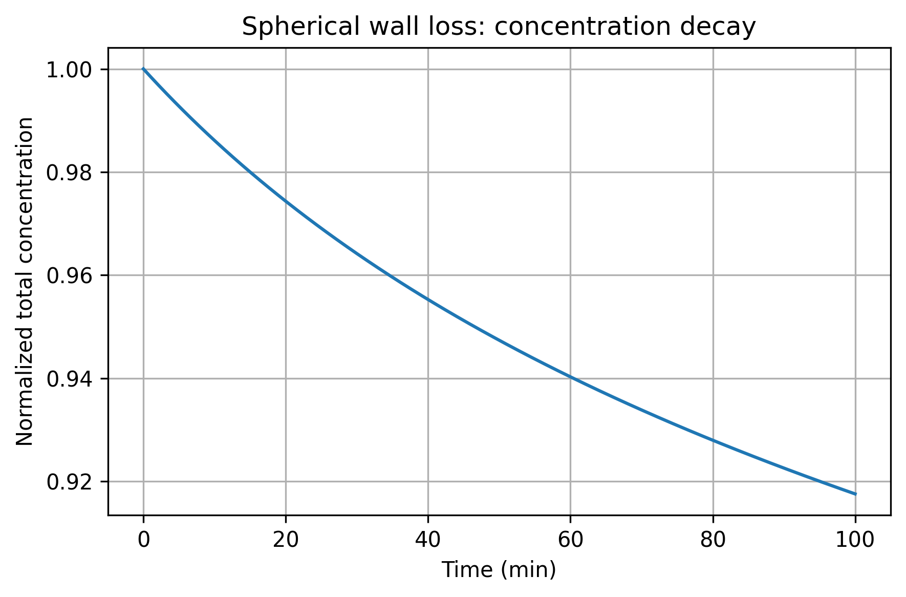
Locate the sizes that were preferentially removed
Section titled “Locate the sizes that were preferentially removed”The second figure retains concentrations in m⁻³ per bin rather than normalizing each spectrum. A change in relative mode heights reflects selective removal; it is not evidence that particles moved between bins. The initial distribution is rebuilt from the same deterministic preset for comparison.
Python · section 6
# Rebuild the initial distribution for comparisoninitial_particle = par.particles.create_lognormal_binned_particle_data(    distribution_type="discrete")
fig, ax = plt.subplots(figsize=(6, 4))
ax.plot(    initial_particle.radii[0],    initial_particle.concentration[0],    label="Initial",)ax.plot(    particle.radii[0],    particle.concentration[0],    label="After wall loss",)
ax.set_xscale("log")ax.set_xlabel("Particle radius (m)")ax.set_ylabel("Number concentration (1/m^3)")ax.set_title("Size distribution before/after wall loss")ax.grid(True)ax.legend()
plt.tight_layout()plt.show()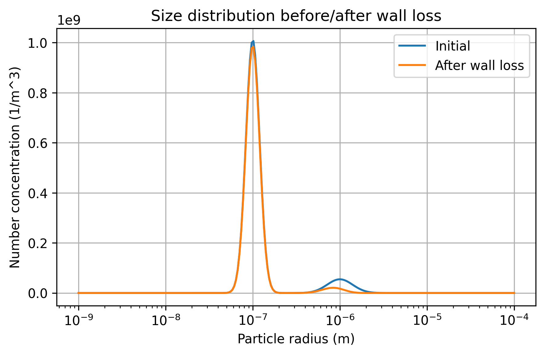
Distinguish a repeated-call sketch from coupled physics
Section titled “Distinguish a repeated-call sketch from coupled physics”The short loop below rebuilds the initial distribution and repeats wall loss for ten 1 s intervals. Despite its legacy comment about condensation, it calls no condensation process. For an actual coupled comparison, use the wall-loss composition example, where the growth and reservoir assumptions are explicit.
Python · section 7
# Pseudo-code: combine condensation and wall lossparticle = par.particles.create_lognormal_binned_particle_data(    distribution_type="discrete")
wall_loss = par.dynamics.SphericalWallLossStrategy(    wall_eddy_diffusivity=1e-3,    chamber_radius=0.5,    distribution_type="discrete",)
# Condensation uses native gas/environment data and explicit process# configuration. For a complete# example that includes gas-particle condensation, see the condensation# tutorials in docs/examples/Dynamics/.
for _ in range(10):    # Apply wall loss to the particle distribution    for _substep in range(sub_steps):        particle = wall_loss.step(            particle=particle,            temperature=T,            pressure=P,            time_step=dt / sub_steps,        )
Carry the interpretation into an experiment
Section titled “Carry the interpretation into an experiment”The saved 100-minute trajectory ends at 1.009×10¹⁰ m⁻³ from 1.100×10¹⁰ m⁻³. It demonstrates a changing spectrum through removal alone, with no individual mass change. Matching the discrete decay formula checks implementation of this update; it does not calibrate the wall-loss model.
A research extension is to infer size-dependent survival from repeated chamber measurements and compare it with the modeled coefficients. First test timestep refinement, then account for dilution and possible coagulation. Those mechanisms can lower number for different reasons and should be separated by their budgets.
Explore this topic: Wall deposition