

Add an external population without changing existing particles
Add an external population without changing existing particles
Section titled “Add an external population without changing existing particles”How should a simulation represent an incoming particle pulse? This example inserts two populations into reserved slots and checks the added material explicitly. It distinguishes an external particle source from nucleation, which transfers material from a modeled precursor reservoir.
The example uses particle-resolved storage, fixed capacity, and unit represented counts. It does not resize arrays, evolve the particles between additions, or define a binned insertion method.
Python · section 1
# In Colab uncomment the following command to install particula:# Install from the repository root: `python -m pip install -e ".[extra]"`import matplotlib.pyplot as pltimport numpy as np
# particula importsimport particula as parfrom particula.particles.slot_management import activate_slots
Reserve capacity around a known initial population
Section titled “Reserve capacity around a known initial population”The 100,000 initial samples have lognormal radius scale 100 nm, geometric standard deviation 1.3, and material density 1500 kg m⁻³. Despite legacy comments mentioning diameter, the samples are used as radii in the mass calculation. Unit counts in 1 cm³ imply number density 10¹¹ m⁻³.
Another 20,000 slots begin with zero mass, count, and charge. They reserve space for two pulses; they are not physical zero-size particles. Temperature and pressure stay at 298.15 K and 101325 Pa, with no gas or dynamical process involved in the insertion.
Python · section 2
gas = par.gas.GasData(    name=["air"],    molar_mass=np.array([0.029]),    concentration=np.array([[1.2]]),    partitioning=np.array([False]),)environment = par.gas.EnvironmentData(    temperature=np.array([298.15]),    pressure=np.array([101325.0]),    saturation_ratio=np.zeros((1, 1)),)np.random.seed(42)
# Generate a particle distribution using a lognormal sample distribution# This distribution has a mean particle diameter (mode) and geometric standard deviation (GSD)particle_sample = par.particles.get_lognormal_sample_distribution(    mode=np.array([100e-9]),  # Mode radius of 100 nm    geometric_standard_deviation=np.array([1.3]),  # GSD    number_of_particles=np.array([1e4]),  # Total number of particles    number_of_samples=100_000,  # Number of samples for particle distribution)
# Calculate the mass of each particle in the sample, assuming density of 1500 kg/m^3particle_mass_sample = (    4 / 3 * np.pi * particle_sample**3 * 1500)  # Particle mass in kg
# Reserve 20,000 free slots for two 10,000-particle additions. Free slots# have exactly zero mass, represented count, and charge.initial_count = particle_mass_sample.sizecapacity = initial_count + 20_000masses = np.zeros((capacity, 1), dtype=np.float64)counts = np.zeros(capacity, dtype=np.float64)masses[:initial_count, 0] = particle_mass_samplecounts[:initial_count] = 1.0resolved_masses = par.particles.create_resolved_particle_data(    masses=masses,    concentration=counts,    density=np.array([1500.0]),    volume=1e-6,  # 1 cm^3 in m^3)aerosol = par.Aerosol(    particles=resolved_masses, gas=gas, environment=environment)
# Print the properties of the atmosphereprint(aerosol)
ParticleData(masses=array([[[9.28905845e-18],
[5.63529914e-18],
[1.04611464e-17],
...,
[0.00000000e+00],
[0.00000000e+00],
[0.00000000e+00]]], shape=(1, 120000, 1)), concentration=array([[1., 1., 1., ..., 0., 0., 0.]], shape=(1, 120000)), charge=array([[0., 0., 0., ..., 0., 0., 0.]], shape=(1, 120000)), density=array([1500.]), volume=array([1.e-06]), distribution_type='particle_resolved', radius_grid=None)
GasData(name=['air'], molar_mass=array([0.029]), concentration=array([[1.2]]), partitioning=array([False]))
EnvironmentData(temperature=array([298.15]), pressure=array([101325.]), saturation_ratio=array([[0.]]))Define the source and account for its inventory
Section titled “Define the source and account for its inventory”Each pulse contains the same sampled 10,000 unit-count particles, with radius scale 1 nm and geometric standard deviation 1.1. These inputs illustrate slot insertion; they are not a physical cluster-formation model at nanometre scales.
Requests specify material masses, represented counts, charges, and the active request length in each box. Activation fills free slots and rejects insufficient capacity before mutation. The checks below require unchanged gas, stable held arrays, and particle material equal to initial inventory plus cumulative injection. After the second pulse, the reserved capacity is exactly exhausted.
Python · section 3
# particles to add
# Generate a particle distribution using a lognormal sample distribution# This distribution has a mean particle diameter (mode) and geometric standard deviation (GSD)particles_to_add = par.particles.get_lognormal_sample_distribution(    mode=np.array([1e-9]),  # Mode radius of 1 nm    geometric_standard_deviation=np.array([1.1]),  # GSD    number_of_particles=np.array([1e4]),  # Total number of particles    number_of_samples=10_000,  # Number of samples for particle distribution)
# Calculate the mass of each particle in the sample, assuming density of 1500 kg/m^3particle_mass_add = (    4 / 3 * np.pi * particles_to_add**3 * 1500)  # Particle mass in kgconcentration_add = np.ones_like(particle_mass_add)

# print shapesprint(f"Particles to add: {particle_mass_add.shape}")
Particles to add: (10000,)Python · section 4
# Only active particles enter the radius histograms.initial_radii = aerosol.particles.radii[0, :initial_count].copy()initial_inventory = np.sum(masses * counts[:, None], axis=0)held_masses = aerosol.particles.massesheld_counts = aerosol.particles.concentrationheld_gas = aerosol.gas.concentration.copy()request_masses = particle_mass_add[None, :, None]request_counts = concentration_add[None, :]request_charge = np.zeros_like(request_counts)requested_counts = np.array([particle_mass_add.size], dtype=np.int32)
radii_after_steps = []for step in (1, 2):    activated = activate_slots(        aerosol.particles,        request_masses=request_masses,        request_concentration=request_counts,        request_charge=request_charge,        requested_counts=requested_counts,    )    np.testing.assert_array_equal(activated, requested_counts)    assert aerosol.particles.masses is held_masses    assert aerosol.particles.concentration is held_counts    np.testing.assert_array_equal(aerosol.gas.concentration, held_gas)    actual = np.sum(        aerosol.particles.masses[0]        * aerosol.particles.concentration[0, :, None],        axis=0,    )    np.testing.assert_allclose(        actual,        initial_inventory + step * particle_mass_add.sum(),        rtol=1e-12,        atol=1e-30,    )    active = aerosol.particles.concentration[0] > 0    radii_after_steps.append(aerosol.particles.radii[0, active].copy())    number_density = aerosol.particles.concentration.sum() / 1e-6    print(f"Number density after step {step}: {number_density:g} m^-3")
radii_after_step_1, radii_after_step_2 = radii_after_stepsnp.testing.assert_array_equal(    par.particles.get_slot_diagnostics(aerosol.particles)[2], [0])
Number density after step 1: 1.1e+11 m^-3
Number density after step 2: 1.2e+11 m^-3Identify an added mode rather than apparent growth
Section titled “Identify an added mode rather than apparent growth”The overlay shows raw counts in radius intervals. With unit weights and fixed volume, dividing those counts by 10⁻⁶ m³ would give number density per bin. No distribution normalization is applied, so the added small-radius population changes the histogram abundance directly.
The saved number densities are 1.1×10¹¹ and 1.2×10¹¹ m⁻³ after the two pulses. The larger seed mode is retained because no growth or collision step occurs between them. The two pulses reuse the same sample, so their fine histogram structure is not independent sampling evidence.
Python · section 5
# Define lognormal bins for particle radius histogrambins_lognormal = np.logspace(-10, -6, 100)
# Create figure for visualizing the histogram of particle radiifig, ax = plt.subplots(figsize=(8, 6))
# Plot radii distribution after step 2bins, edges = np.histogram(radii_after_step_2, bins=bins_lognormal)ax.bar(    edges[:-1],    bins,    width=np.diff(edges),    align="edge",    label="After 2 steps",    alpha=0.6,)# Plot radii distribution after step 1
bins, edges = np.histogram(radii_after_step_1, bins=bins_lognormal)ax.bar(    edges[:-1],    bins,    width=np.diff(edges),    align="edge",    label="After 1 step",    alpha=0.5,)
# Plot initial radii distributionbins, edges = np.histogram(initial_radii, bins=bins_lognormal)ax.bar(    edges[:-1],    bins,    width=np.diff(edges),    align="edge",    label="Initial",    alpha=0.4,    edgecolor="black",)
# Set axes to logarithmic scale for x-axis (particle radius)ax.set_xscale("log")ax.set_yscale("log")
# Add labels and legendax.set_xlabel("Radius (m)")ax.set_ylabel("Number of particles")plt.legend()
# Show the plotplt.show()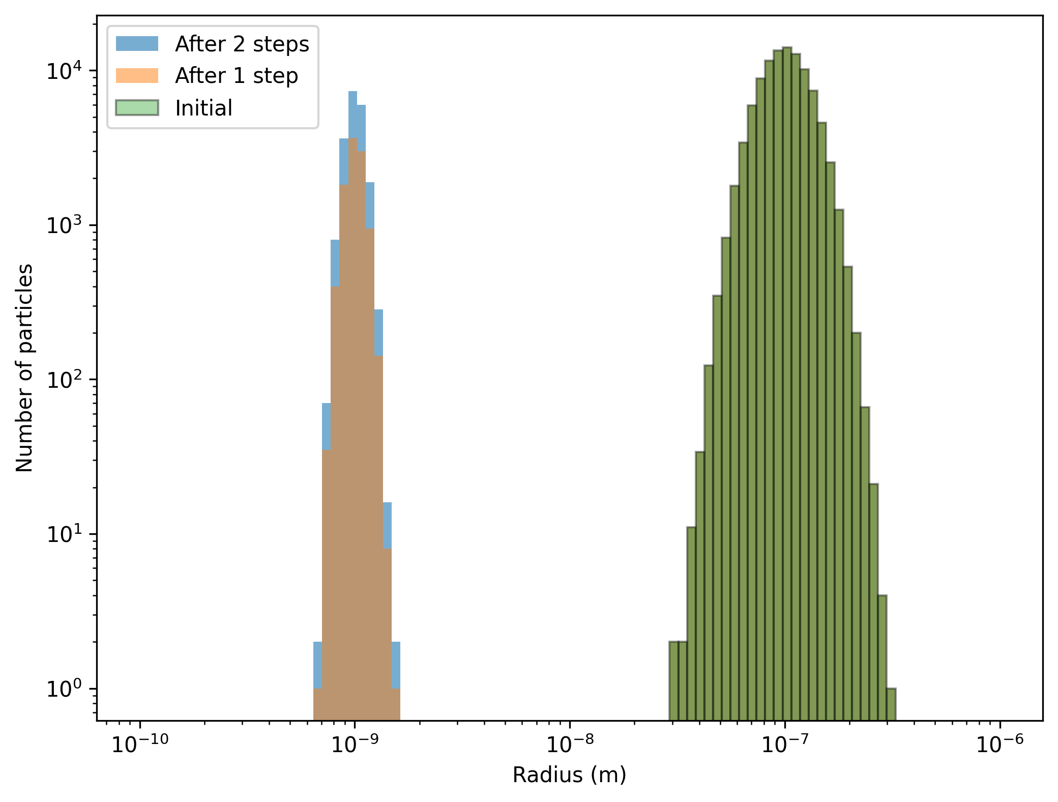
Turn insertion into a source experiment
Section titled “Turn insertion into a source experiment”The result establishes controlled external additions with an explicit material budget and finite capacity. It does not establish what the new particles do after entering the system.
To study whether fresh nuclei survive in an existing aerosol, add a growth and collision interval between pulses. Compare surviving small-particle number, material inventory, and required slot capacity while refining the interval. For a tracer or source label, define its birth and merging behavior using the registered-field example, rather than assuming array position remains a particle identity.
Explore this topic: Custom processes and fields