

A compact comparison of bin totals and radius densities
A compact comparison of bin totals and radius densities
Section titled “A compact comparison of bin totals and radius densities”Can different-looking concentration arrays describe the same aerosol? This example builds a PMF and a PDF from matching physical inputs, advances each for 200 s, and converts units before comparing. It is a small starting point for learning how representation enters a numerical comparison.
The distribution-measure example explains why bin width matters. The longer coagulation comparison uses a broader grid and a higher abundance to make evolution more visible.
Python · section 1
# In Colab uncomment the following command to install particula:# Install from the repository root: `python -m pip install -e ".[extra]"`import matplotlib.pyplot as pltimport numpy as npimport particula as parfrom scipy.integrate import trapezoidHold the intended population fixed
Section titled “Hold the intended population fixed”Both representations use 140 radius nodes from 10 nm–1 µm, lognormal radius scale 120 nm, geometric standard deviation 1.5, and target number density 8×10⁸ m⁻³. Density is 1000 kg m⁻³ at 298.15 K and 101325 Pa. The PMF stores bin totals (m⁻³); the PDF stores density per radius (m⁻⁴). Independent copies of gas and environment isolate the two trajectories.
Python · section 2
# Shared grid (modest resolution)radius_bins = np.logspace(-8, -6, 140)  # m
# Lognormal parameters (kept small for speed)mode = np.array([120e-9])gsd = np.array([1.5])number_conc = np.array([8e8])  # m^-3 total
# PMF (number per bin)concentration_pmf = par.particles.get_lognormal_pmf_distribution(    x_values=radius_bins,    mode=mode,    geometric_standard_deviation=gsd,    number_of_particles=number_conc,)
# PDF (number per size)concentration_pdf = par.particles.get_lognormal_pdf_distribution(    x_values=radius_bins,    mode=mode,    geometric_standard_deviation=gsd,    number_of_particles=number_conc,)
# Native ambient environment. GasData requires a species axis, so a# zero-concentration, non-partitioning carrier fills that axis. Coagulation# does not consume it; ambient pressure is specified independently.environment = par.gas.EnvironmentData(    temperature=np.array([298.15]),    pressure=np.array([101325.0]),    saturation_ratio=np.zeros((1, 1)),)gas = par.gas.GasData(    name=["carrier"],    molar_mass=np.array([0.02897]),    partitioning=np.array([False]),    concentration=np.zeros((1, 1)),)
# PMF particlesparticles_pmf = par.particles.create_particle_data_from_radii(    radii=radius_bins,    concentration=concentration_pmf,    distribution_type="discrete",    density=1000.0,)
aerosol_pmf = par.Aerosol(    particles=particles_pmf, gas=gas.copy(), environment=environment.copy())
# PDF particlesparticles_pdf = par.particles.create_particle_data_from_radii(    radii=radius_bins,    concentration=concentration_pdf,    distribution_type="continuous_pdf",    density=1000.0,)
aerosol_pdf = par.Aerosol(    particles=particles_pdf, gas=gas.copy(), environment=environment.copy())
Match each strategy to its concentration measure
Section titled “Match each strategy to its concentration measure”Both strategies use Brownian collisions. Selecting discrete or
continuous_pdf controls the numerical interpretation; it does not convert
an array from one measure to the other.
Python · section 3
coagulation_pmf = par.dynamics.Coagulation(    coagulation_strategy=(        par.dynamics.BrownianCoagulationBuilder()        .set_distribution_type("discrete")        .build()    ))
coagulation_pdf = par.dynamics.Coagulation(    coagulation_strategy=(        par.dynamics.BrownianCoagulationBuilder()        .set_distribution_type("continuous_pdf")        .build()    ))
print(coagulation_pmf)print(coagulation_pdf)
<particula.dynamics.particle_process.Coagulation object at 0x7f97fc16bbc0>
<particula.dynamics.particle_process.Coagulation object at 0x7f974d5f3110>Advance equal physical time
Section titled “Advance equal physical time”Each process advances 200 s with ten substeps. Copied concentration arrays retain before/after snapshots despite in-place evolution. These modest conditions can produce very small visible changes, so a later accuracy study should compare numerical diagnostics as well as curves.
Python · section 4
time_step = 200  # secondssub_steps = 10
# PMF runpmf_before = aerosol_pmf.particles.concentration[0].copy()aerosol_pmf_after = coagulation_pmf.execute(    aerosol_pmf, time_step=time_step, sub_steps=sub_steps)pmf_after = aerosol_pmf_after.particles.concentration[0].copy()
# PDF runpdf_before = aerosol_pdf.particles.concentration[0].copy()aerosol_pdf_after = coagulation_pdf.execute(    aerosol_pdf, time_step=time_step, sub_steps=sub_steps)pdf_after = aerosol_pdf_after.particles.concentration[0].copy()
Convert before judging agreement
Section titled “Convert before judging agreement”Radius-dependent widths turn PDF density into per-bin number and vice versa. The printed totals use a sum for PMF and a trapezoidal integral for PDF; both round to 8×10⁸ m⁻³ in the saved run. Agreement at that precision checks initial abundance, not equality of every bin or subsequent mass conservation.
Python · section 5
pdf_as_pmf_before = par.particles.get_pdf_distribution_in_pmf(    x_array=radius_bins, distribution=pdf_before, to_pdf=False)pdf_as_pmf_after = par.particles.get_pdf_distribution_in_pmf(    x_array=radius_bins, distribution=pdf_after, to_pdf=False)
pmf_as_pdf_before = par.particles.get_pdf_distribution_in_pmf(    x_array=radius_bins, distribution=pmf_before, to_pdf=True)pmf_as_pdf_after = par.particles.get_pdf_distribution_in_pmf(    x_array=radius_bins, distribution=pmf_after, to_pdf=True)
# Quick consistency checknumber_pmf = pmf_before.sum()number_pdf = trapezoid(pdf_before, x=radius_bins)print(f"Total number PMF: {number_pmf:.2e} m^-3")print(f"Total number PDF: {number_pdf:.2e} m^-3 (integrated)")
Total number PMF: 8.00e+08 m^-3
Total number PDF: 8.00e+08 m^-3 (integrated)Use both panels to identify a measure mismatch
Section titled “Use both panels to identify a measure mismatch”The first panel puts all curves in PMF units; the second puts them in PDF units. Compare initial curves within a panel before assessing the evolved curves. Raw peak heights across panels are not comparable because the vertical units differ. Logarithmic radius spacing does not turn a per-radius PDF into a per-log-radius density.
Python · section 6
fig, ax = plt.subplots(figsize=(8, 5))ax.plot(radius_bins, pmf_before, label="PMF before", color="tab:blue")ax.plot(radius_bins, pmf_after, label="PMF after", color="tab:orange")ax.plot( radius_bins, pdf_as_pmf_before, label="PDF→PMF before", color="tab:green", linestyle="--",)ax.plot( radius_bins, pdf_as_pmf_after, label="PDF→PMF after", color="tab:red", linestyle="--",)ax.set_xscale("log")ax.set_xlabel("Particle radius (m)")ax.set_ylabel(r"Number concentration ($m^{-3}$)")ax.set_title("PMF vs PDF coagulation (converted to PMF units)")ax.legend()ax.grid(alpha=0.3)plt.show()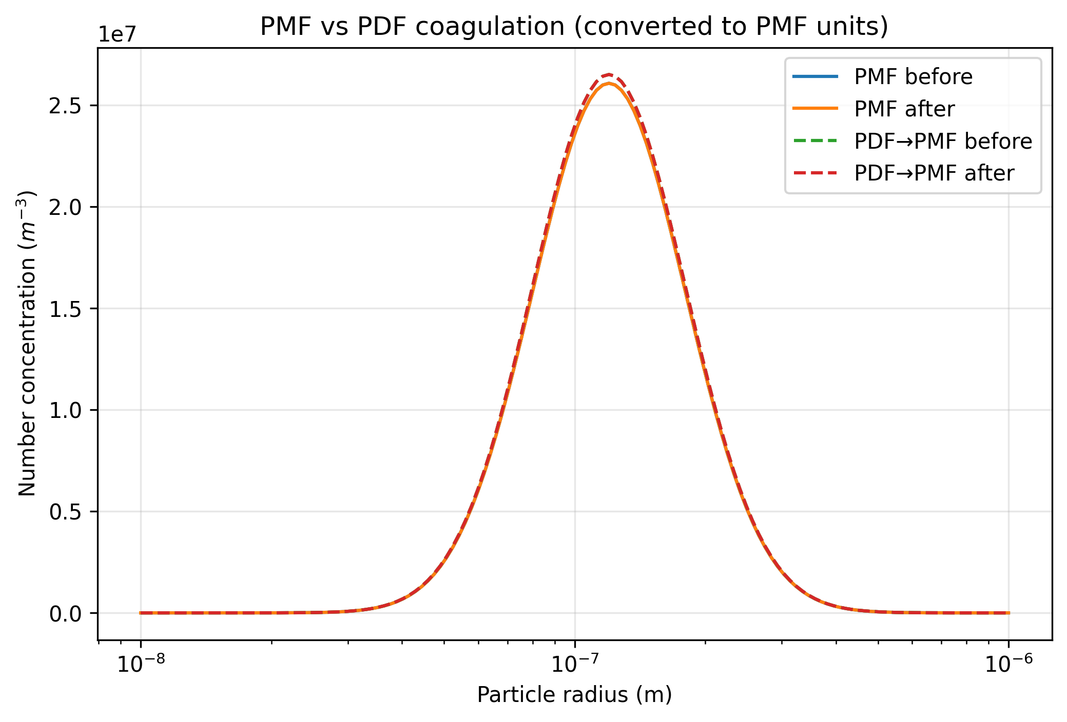
Python · section 7
fig, ax = plt.subplots(figsize=(8, 5))ax.plot( radius_bins, pmf_as_pdf_before, label="PMF→PDF before", color="tab:blue")ax.plot( radius_bins, pmf_as_pdf_after, label="PMF→PDF after", color="tab:orange")ax.plot( radius_bins, pdf_before, label="PDF before", color="tab:green", linestyle="--",)ax.plot( radius_bins, pdf_after, label="PDF after", color="tab:red", linestyle="--")ax.set_xscale("log")ax.set_xlabel("Particle radius (m)")ax.set_ylabel(r"PDF concentration ($m^{-4}$)")ax.set_title("PMF vs PDF coagulation (PDF units)")ax.legend()ax.grid(alpha=0.3)plt.show()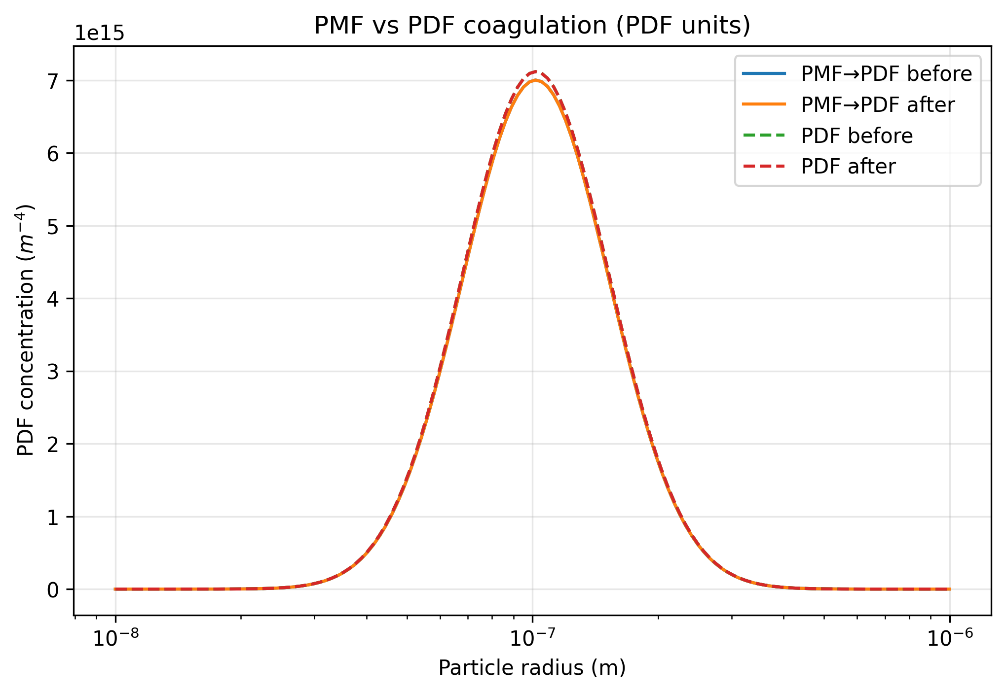
From matching plots to a scientific test
Section titled “From matching plots to a scientific test”The conversions make the two simulations comparable. They do not prove either method accurate. To test sensitivity, refine grid resolution and extent, then substeps, and track total number and mass alongside the converted spectrum.
If your research concerns the survival of a size-selected population, compare integrated number within that radius interval rather than only the total. The time-evolution example shows how to extend a matched comparison through time.
Native construction preserves the generated arrays. Finite-grid coagulation can exhibit mass drift; a successful run and a visual overlay are not conservation or convergence tests.
Explore this topic: Comparing representations