Skip to content

Follow organic uptake onto seeds during imposed cooling

Download Python script

Follow organic uptake onto seeds during imposed cooling

Section titled “Follow organic uptake onto seeds during imposed cooling”

How can cooling alter gas–particle partitioning while collisions change particle size? This example follows 24 organic species around a supplied seed population, applying condensation and Brownian coagulation under a prescribed temperature history. It connects volatility assumptions to mass and size diagnostics.

Despite the historical filename, this is not a soot-formation chemistry model. There is no nucleation, reaction network, carbonization, oxidation, or aggregate morphology. Fullerene-labeled seeds already exist at the start. Material tables and cooling are illustrative, not a calibrated flame or plume. Read organic partitioning and resolved coagulation for the separate mechanisms.

Python · section 1
# 🚧 Install Particula if you're running this in Google Colab
# Remove the comment below to enable installation
# Install from the repository root: `python -m pip install -e ".[extra]"`
# 📦 Import necessary libraries
import copy # to safely duplicate Python objects
from typing import Union
import matplotlib.pyplot as plt # for plotting
import numpy as np # numerical tools
import particula as par # the main Particula package
from matplotlib.colors import LogNorm
from numpy.typing import NDArray
from particula.dynamics.condensation.species_mapping import (
CondensationSpeciesMap,
)
from tqdm import tqdm # optional: for progress bars during simulation
# 🎨 Set default plot styling using Tailwind-inspired colors from Particula
TAILWIND = par.util.colors.TAILWIND
base_color = TAILWIND["gray"]["600"]
plt.rcParams.update(
{
"text.color": base_color,
"axes.labelcolor": base_color,
"figure.figsize": (5, 4),
"font.size": 14,
"axes.edgecolor": base_color,
"xtick.color": base_color,
"ytick.color": base_color,
"pdf.fonttype": 42,
"ps.fonttype": 42,
}
)
# 🌌 Define the colors for the chemical species involved in the simulation
color_list = (
# 1–2 ring aromatics (amber)
[
TAILWIND["amber"][shade]
for shade in ["400", "500", "600", "700", "800", "900"]
]
+
# 3–4 ring PAHs (sky)
[
TAILWIND["sky"][shade]
for shade in [
"300",
"400",
"500",
"600",
"700",
"800",
"900",
"200",
]
]
+
# 5–7 ring PAHs (rose)
[
TAILWIND["rose"][shade]
for shade in [
"300",
"400",
"500",
"600",
"700",
"800",
"900",
"200",
]
]
+
# Extra-large PAH surrogate (slate)
[TAILWIND["slate"]["800"]]
+
# Fullerene (indigo)
[TAILWIND["indigo"]["700"]]
)

Define the species and audit the property lookup

Section titled “Define the species and audit the property lookup”

The list spans small aromatics, PAHs, and a fullerene seed label. Supplied gas mass fractions are normalized to one; they are not tied here to a measured emission profile. The utility resolves names before retrieving properties. A returned numerical value does not establish a correct identity or validity at flame temperatures; inspect the resolved identifiers and property methods before using this as a material model.

Molar masses are kg/mol and densities kg/m³. The displayed standard-condition properties initialize part of the model; they do not mean all properties are updated consistently during cooling.

Python · section 2
# Define species list grouped by volatility
list_of_chemicals = [
# 1–2-ring aromatics (gas-phase precursors, ~65%)
"Benzene",
"Toluene",
"Ethylbenzene",
"p-Xylene",
"Styrene",
"Indene",
# 2–4-ring PAHs (semi-volatile, ~35%)
"Naphthalene",
"Acenaphthylene",
"Acenaphthene",
"Anthracene",
"Fluoranthene",
"Pyrene",
"Chrysene",
"Benzo[a]anthracene",
# 5–7-ring PAHs (low volatility)
"Benzo[b]fluoranthene",
"Benzo[k]fluoranthene",
"Benzo[a]pyrene",
"Perylene",
"Benzo[ghi]perylene",
"Indeno[1,2,3-cd]pyrene",
"Dibenzo[a,h]anthracene",
"Coronene",
# Optional ≥7-ring surrogate and soot seed
"Ovalene",
"Fullerene",
]
# Initial mass fractions (normalized)
initial_mass_fractions = np.array(
[
# ------- 1–2-ring aromatics (~65%)
0.20,
0.15,
0.10,
0.10,
0.05,
0.05,
# ------- 2–4-ring PAHs (~35%)
0.12068966,
0.01931034,
0.01448276,
0.01448276,
0.02896552,
0.02896552,
0.01448276,
0.00965517,
# ------- 5–7-ring PAHs
0.01448276,
0.00965517,
0.00965517,
0.00724138,
0.00724138,
0.00482759,
0.00337931,
0.00241379,
0.00144828,
0.00072414,
],
dtype=np.float64,
)
# Normalize to sum to 1
initial_mass_fractions /= np.sum(initial_mass_fractions)
# Initialize property arrays
density_array = np.array([])
molar_mass_array = np.array([])
surface_tension_array = np.array([])
cas_name = []
chemical_dict = {}
# Retrieve and store properties
for chem in list_of_chemicals:
cas = par.util.get_chemical_search(chem)
print(f"{chem}: {cas}")
chemical_dict[chem] = par.util.get_chemical_stp_properties(cas)
molar_mass_array = np.append(
molar_mass_array, chemical_dict[chem]["molar_mass"]
)
density_array = np.append(density_array, chemical_dict[chem]["density"])
surface_tension_array = np.append(
surface_tension_array, chemical_dict[chem]["surface_tension"]
)
cas_name.append(cas)
# Display property summary
for chem, props in chemical_dict.items():
print(f"{chem}:")
print(f" Molar Mass: {props['molar_mass']:.4f} kg/mol")
print(f" Density: {props['density']:.2f} kg/m³")
print(f" Surface Tension: {props['surface_tension']} N/m")
print(f" Vapor Pressure: {props['pure_vapor_pressure']} Pa\n")
Benzene: Benzene
Toluene: Toluene
Ethylbenzene: Ethylbenzene
p-Xylene: p-Xylene
Styrene: Styrene
Indene: Indene
Naphthalene: Naphthalene
Acenaphthylene: Acenaphthylene
Acenaphthene: Acenaphthene
Anthracene: Anthracene
Fluoranthene: Fluoranthene
Pyrene: Pyrene
Chrysene: Chrysene
Benzo[a]anthracene: Benzo[a]anthracene
Benzo[b]fluoranthene: Benzo[b]fluoranthene
Benzo[k]fluoranthene: Benzo[k]fluoranthene
Benzo[a]pyrene: Benzo[a]pyrene
Perylene: Perylene
Benzo[ghi]perylene: Benzo[ghi]perylene
Indeno[1,2,3-cd]pyrene: Indeno[1,2,3-cd]pyrene
Dibenzo[a,h]anthracene: Dibenzo[a,h]anthracene
Coronene: Coronene
Ovalene: Ovalene
Fullerene: Fullerene
Benzene:
  Molar Mass: 0.0781 kg/mol
  Density: 873.76 kg/m³
  Surface Tension: 0.028206202466830844 N/m
  Vapor Pressure: 12695.06760788906 Pa
Toluene:
  Molar Mass: 0.0921 kg/mol
  Density: 862.34 kg/m³
  Surface Tension: 0.027906333880214882 N/m
  Vapor Pressure: 3799.2916085833076 Pa
Ethylbenzene:
  Molar Mass: 0.1062 kg/mol
  Density: 862.64 kg/m³
  Surface Tension: 0.028519673106300977 N/m
  Vapor Pressure: 1278.8635512049998 Pa
p-Xylene:
  Molar Mass: 0.1062 kg/mol
  Density: 856.84 kg/m³
  Surface Tension: 0.02780489434006062 N/m
  Vapor Pressure: 1177.6548935579035 Pa
Styrene:
  Molar Mass: 0.1041 kg/mol
  Density: 900.52 kg/m³
  Surface Tension: 0.030530851011226136 N/m
  Vapor Pressure: 821.533882502462 Pa
Indene:
  Molar Mass: 0.1162 kg/mol
  Density: 957.15 kg/m³
  Surface Tension: 0.019075436088789817 N/m
  Vapor Pressure: 225.95221357669246 Pa
Naphthalene:
  Molar Mass: 0.1282 kg/mol
  Density: 1120.20 kg/m³
  Surface Tension: 0.041817073351975 N/m
  Vapor Pressure: 42.179417148049055 Pa
Acenaphthylene:
  Molar Mass: 0.1522 kg/mol
  Density: 1113.30 kg/m³
  Surface Tension: 0.04143820989061258 N/m
  Vapor Pressure: 2.83294928153961 Pa
Acenaphthene:
  Molar Mass: 0.1542 kg/mol
  Density: 972.47 kg/m³
  Surface Tension: 0.0385194992687528 N/m
  Vapor Pressure: 1.9222921879309003 Pa
Anthracene:
  Molar Mass: 0.1782 kg/mol
  Density: 1106.97 kg/m³
  Surface Tension: 0.04831768955111898 N/m
  Vapor Pressure: 0.362912065174679 Pa
Fluoranthene:
  Molar Mass: 0.2023 kg/mol
  Density: 1116.91 kg/m³
  Surface Tension: 0.046639222539928284 N/m
  Vapor Pressure: 0.0008003908764101553 Pa
Pyrene:
  Molar Mass: 0.2023 kg/mol
  Density: 1158.87 kg/m³
  Surface Tension: 0.04893250644932069 N/m
  Vapor Pressure: 5.1375589253832836e-05 Pa
Chrysene:
  Molar Mass: 0.2283 kg/mol
  Density: 1077.02 kg/m³
  Surface Tension: 0.04985254377774797 N/m
  Vapor Pressure: 2.6846652822105422e-05 Pa
Benzo[a]anthracene:
  Molar Mass: 0.2283 kg/mol
  Density: 1203.04 kg/m³
  Surface Tension: 0.05157277097913564 N/m
  Vapor Pressure: 5.569142923796036e-05 Pa
Benzo[b]fluoranthene:
  Molar Mass: 0.2523 kg/mol
  Density: 1150.91 kg/m³
  Surface Tension: 0.050472914014624566 N/m
  Vapor Pressure: 4.393050525936658e-06 Pa
Benzo[k]fluoranthene:
  Molar Mass: 0.2523 kg/mol
  Density: 1171.82 kg/m³
  Surface Tension: 0.04582707666133075 N/m
  Vapor Pressure: 0.0005678510119370869 Pa
Benzo[a]pyrene:
  Molar Mass: 0.2523 kg/mol
  Density: 1186.70 kg/m³
  Surface Tension: 0.04608662360222815 N/m
  Vapor Pressure: 0.0004701165050824623 Pa
Perylene:
  Molar Mass: 0.2523 kg/mol
  Density: 1145.59 kg/m³
  Surface Tension: 0.0461198819597169 N/m
  Vapor Pressure: 0.00045887128419603445 Pa
Benzo[ghi]perylene:
  Molar Mass: 0.2763 kg/mol
  Density: 1175.67 kg/m³
  Surface Tension: 0.04702177589801932 N/m
  Vapor Pressure: 7.126539938521257e-05 Pa
Indeno[1,2,3-cd]pyrene:
  Molar Mass: 0.2763 kg/mol
  Density: 1213.67 kg/m³
  Surface Tension: 0.04679231808084244 N/m
  Vapor Pressure: 8.535388889438557e-05 Pa
Dibenzo[a,h]anthracene:
  Molar Mass: 0.2783 kg/mol
  Density: 1172.69 kg/m³
  Surface Tension: 0.04880049181278169 N/m
  Vapor Pressure: 9.217001932898797e-06 Pa
Coronene:
  Molar Mass: 0.3004 kg/mol
  Density: 1116.06 kg/m³
  Surface Tension: 0.04653055920308998 N/m
  Vapor Pressure: 3.467366635539694e-05 Pa
Ovalene:
  Molar Mass: 0.3985 kg/mol
  Density: 1240.61 kg/m³
  Surface Tension: 0.07585556520479782 N/m
  Vapor Pressure: 7.325250517430775e-14 Pa
Fullerene:
  Molar Mass: 0.7206 kg/mol
  Density: 1441.72 kg/m³
  Surface Tension: 0.040270320922924846 N/m
  Vapor Pressure: 4.1068395355330673e-17 Pa

Build temperature-dependent tables and expose their limits

Section titled “Build temperature-dependent tables and expose their limits”

There are 5000 sampled particles at 10⁷ cm⁻³, represented in 5×10⁻¹⁰ m³. The total initial organic gas concentration is 5×10⁻⁵ kg/m³. These chosen conditions are not qualified as a particular combustion source.

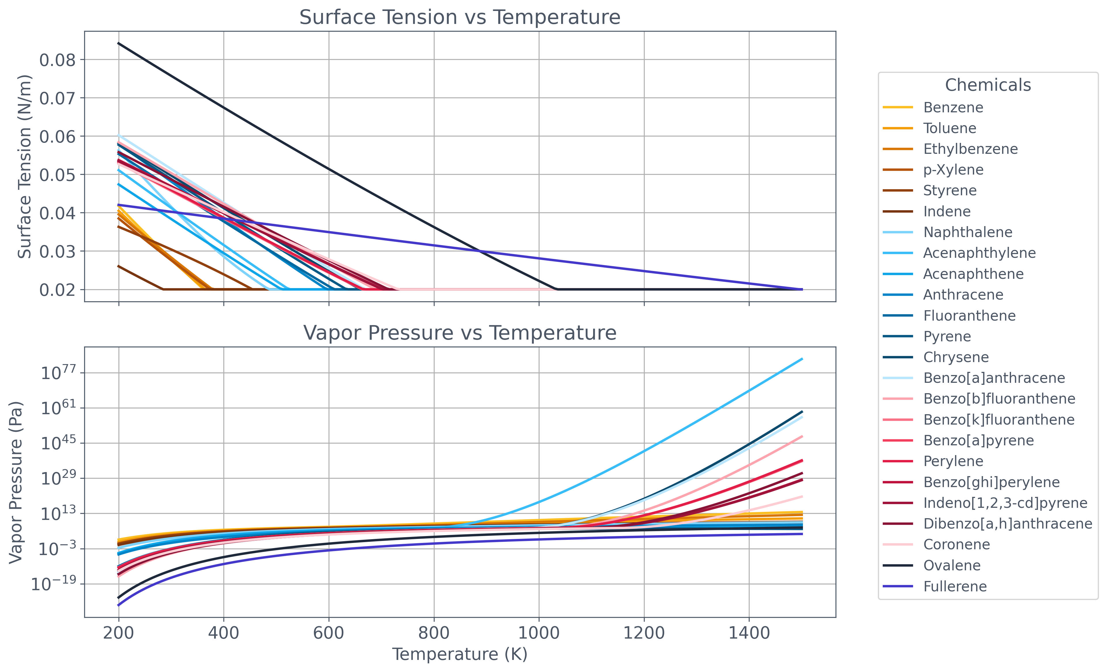
Vapor-pressure and surface-tension tables use 200 points from 200–1500 K. Surface tensions replace NaNs and impose a 0.02 N/m floor. Those numerical substitutions are model assumptions, not measurements at high temperature. The separately plotted vapor-pressure array is clipped after the strategies are constructed; that display operation should not be read as proof of the strategies’ underlying property validity. The charts help locate strong trends and questionable extrapolations; they do not establish chemical stability.

Python · section 3
# Reproducible initial sampling. Coagulation owns a separate random generator;
# trajectories are stochastic and are not asserted equal across runs.
np.random.seed(100)
# Simulation parameters
number_of_samples = 5_000 # Simulated particles
total_number_per_cm3 = 10_000_000 # #/cm³
simulation_volume = number_of_samples / total_number_per_cm3 * 1e-6 # m³
# Initial gas phase loading and temperature
total_mass_gas_phase = 5e-5 # kg/m³
temperature = 1200 # Initial gas temperature [K]
# Temperature range for property tables
temperature_range_table = np.linspace(200, 1500, 200)
# Preallocate property tables
vapor_pressure_strategy_list = []
surface_tension_table = np.zeros(
(len(temperature_range_table), len(list_of_chemicals))
)
vapor_pressure_table = np.zeros(
(len(temperature_range_table), len(list_of_chemicals))
)
# Loop through chemicals to build property tables
for chem_i in list(chemical_dict.keys()):
idx = list_of_chemicals.index(chem_i)
# Vapor pressure vs temperature
vapor_pressure_temp = par.util.get_chemical_vapor_pressure(
chemical_identifier=chem_i,
temperature=temperature_range_table,
)
vapor_pressure_table[:, idx] = vapor_pressure_temp
vapor_pressure_strategy = (
par.gas.TableVaporPressureBuilder()
.set_temperature_table(temperature_range_table, "K")
.set_vapor_pressure_table(vapor_pressure_temp, "Pa")
.build()
)
vapor_pressure_strategy_list.append(vapor_pressure_strategy)
# Surface tension vs temperature
surface_tension_temp = par.util.get_chemical_surface_tension(
chemical_identifier=chem_i,
temperature=temperature_range_table,
)
surface_tension_table[:, idx] = surface_tension_temp
# Clean up NaNs or extreme values
surface_tension_table = np.nan_to_num(surface_tension_table, nan=2e-2)
surface_tension_table = np.clip(surface_tension_table, a_min=2e-2, a_max=None)
vapor_pressure_table = np.clip(vapor_pressure_table, a_min=1e-50, a_max=1e100)
# 🔍 Plot property tables
fig, ax = plt.subplots(2, 1, figsize=(10, 8), sharex=True)
for i, chem in enumerate(list_of_chemicals):
ax[0].plot(
temperature_range_table,
surface_tension_table[:, i],
label=chem,
linewidth=2,
color=color_list[i],
)
ax[1].plot(
temperature_range_table,
vapor_pressure_table[:, i],
label=chem,
linewidth=2,
color=color_list[i],
)
ax[0].set_ylabel("Surface Tension (N/m)")
ax[0].set_title("Surface Tension vs Temperature")
ax[0].grid()
ax[1].set_yscale("log")
ax[1].set_ylabel("Vapor Pressure (Pa)")
ax[1].set_xlabel("Temperature (K)")
ax[1].set_title("Vapor Pressure vs Temperature")
ax[1].grid()
# Combined legend
fig.legend(
list_of_chemicals,
loc="center left",
bbox_to_anchor=(1.02, 0.5),
title="Chemicals",
fontsize="small",
)
plt.tight_layout(rect=(0, 0, 1, 1))
plt.show()
Follow organic uptake onto seeds during imposed cooling: saved scientific figure
Follow organic uptake onto seeds during imposed cooling · saved execution output

Put the available material into a closed gas inventory

Section titled “Put the available material into a closed gas inventory”

Each normalized fraction multiplies the total gas mass concentration. Native GasData stores that ordered inventory, while EnvironmentData stores pressure and temperature. The initial 1200 K value is replaced by the forcing below. The parcel volume and pressure remain fixed: prescribed cooling here does not also simulate expansion, entrainment, or dilution of material.

Python · section 4
# Compute gas-phase concentration [kg/m³]
concentration_gas = initial_mass_fractions * total_mass_gas_phase
# Initialize gas-phase species with vapor pressure strategy
gas_species = par.gas.GasData(
name=list_of_chemicals,
molar_mass=molar_mass_array.copy(),
partitioning=np.ones(len(list_of_chemicals), dtype=bool),
concentration=concentration_gas[None, :].copy(),
)
environment = par.gas.EnvironmentData(
temperature=np.array([float(temperature)]),
pressure=np.array([101325.0]),
saturation_ratio=np.zeros((1, len(list_of_chemicals))),
)

Supply the condensation sites rather than create them

Section titled “Supply the condensation sites rather than create them”

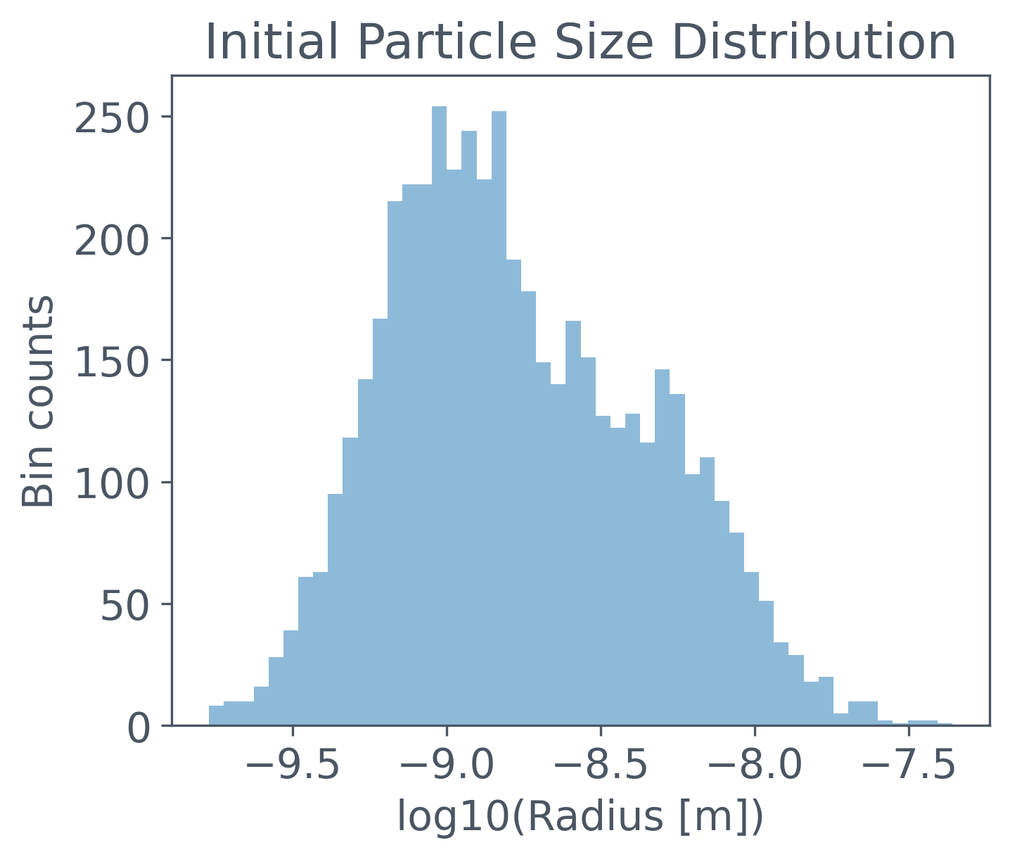
Two lognormal seed-radius modes at 1 and 5 nm, both with geometric standard deviation 1.8, populate the resolved sample. All initial particle mass occupies the final, fullerene-labeled lane. The initial histogram counts particles per log-radius bin; it does not show a nucleation rate.

Ideal molar activity and a mass-weighted surface treatment are imposed. The seed has a separate phase label from the other organics. At the smallest sizes, continuum surface and transport assumptions themselves need scrutiny. The species-inventory helper includes gas mass times represented volume, so later closed material comparisons use kg per species.

Python · section 5
# Generate bi-modal seed particle distribution [m]
radii_seeds = par.particles.get_lognormal_sample_distribution(
mode=np.array([1e-9, 5e-9]), # 1 nm and 5 nm modes
geometric_standard_deviation=np.array([1.8, 1.8]),
number_of_particles=np.array([1, 0.5]), # relative mode strength
number_of_samples=number_of_samples,
)
# Calculate seed mass assuming all are pure fullerene
mass_seeds = (4 / 3) * np.pi * (radii_seeds**3) * density_array[-1]
# Initialize mass speciation matrix: all mass in fullerene (last index)
mass_speciation = np.zeros((number_of_samples, len(list_of_chemicals)))
mass_speciation[:, -1] = mass_seeds
# Activity strategy (ideal molar)
activity_strategy = (
par.particles.ActivityIdealMolarBuilder()
.set_molar_mass(molar_mass_array, "kg/mol")
.build()
)
# Phase indices: all condensed except the seed
phases = np.ones_like(density_array)
phases[-1] = 0 # last species (fullerene) is seed, not condensing
# Surface tension strategy (temperature-dependent)
surface_strategy = (
par.particles.SurfaceStrategyMassBuilder()
.set_surface_tension(surface_tension_array, "N/m")
.set_density(density_array, "kg/m^3")
.set_phase_index(phases)
.set_surface_tension_table(surface_tension_table, "N/m")
.set_temperature_table(temperature_range_table, "K")
.build()
)
# Build the particle representation
resolved_masses = par.particles.create_resolved_particle_data(
masses=mass_speciation,
density=density_array,
volume=simulation_volume,
)
aerosol = par.Aerosol(
particles=resolved_masses, gas=gas_species, environment=environment
)
def species_inventory(aero):
"""Independent extensive species accounting including gas, kg."""
return np.sum(
aero.particles.masses * aero.particles.concentration[..., None], axis=1
) + (aero.gas.concentration * aero.particles.volume[:, None])
initial_inventory = species_inventory(aerosol)
print(aerosol)
# 📊 Plot the initial size distribution
fig, ax = plt.subplots()
ax.hist(np.log10(resolved_masses.radii[0]), bins=50, alpha=0.5)
ax.set_xlabel("log10(Radius [m])")
ax.set_ylabel("Bin counts")
ax.set_title("Initial Particle Size Distribution")
plt.show()
ParticleData(masses=array([[[0.00000000e+00, 0.00000000e+00, 0.00000000e+00, ...,
         0.00000000e+00, 0.00000000e+00, 2.76038459e-25],
        [0.00000000e+00, 0.00000000e+00, 0.00000000e+00, ...,
         0.00000000e+00, 0.00000000e+00, 4.61302337e-23],
        [0.00000000e+00, 0.00000000e+00, 0.00000000e+00, ...,
         0.00000000e+00, 0.00000000e+00, 3.40787211e-23],
        ...,
        [0.00000000e+00, 0.00000000e+00, 0.00000000e+00, ...,
         0.00000000e+00, 0.00000000e+00, 2.41594302e-21],
        [0.00000000e+00, 0.00000000e+00, 0.00000000e+00, ...,
         0.00000000e+00, 0.00000000e+00, 2.75849762e-22],
        [0.00000000e+00, 0.00000000e+00, 0.00000000e+00, ...,
         0.00000000e+00, 0.00000000e+00, 4.70283383e-22]]],
      shape=(1, 5000, 24)), concentration=array([[1., 1., 1., ..., 1., 1., 1.]], shape=(1, 5000)), charge=array([[0., 0., 0., ..., 0., 0., 0.]], shape=(1, 5000)), density=array([ 873.75728163,  862.3405711 ,  862.64081188,  856.84076464,
        900.52250717,  957.14688387, 1120.20362048, 1113.30161014,
        972.4737836 , 1106.97030513, 1116.91442516, 1158.870467  ,
       1077.0209774 , 1203.03774275, 1150.90754397, 1171.8180837 ,
       1186.69738114, 1145.58749368, 1175.67352836, 1213.67033011,
       1172.68838322, 1116.05748879, 1240.60653023, 1441.72368025]), volume=array([5.e-10]), distribution_type='particle_resolved', radius_grid=None)
GasData(name=['Benzene', 'Toluene', 'Ethylbenzene', 'p-Xylene', 'Styrene', 'Indene', 'Naphthalene', 'Acenaphthylene', 'Acenaphthene', 'Anthracene', 'Fluoranthene', 'Pyrene', 'Chrysene', 'Benzo[a]anthracene', 'Benzo[b]fluoranthene', 'Benzo[k]fluoranthene', 'Benzo[a]pyrene', 'Perylene', 'Benzo[ghi]perylene', 'Indeno[1,2,3-cd]pyrene', 'Dibenzo[a,h]anthracene', 'Coronene', 'Ovalene', 'Fullerene'], molar_mass=array([0.07811184, 0.09213842, 0.106165  , 0.106165  , 0.10414912,
       0.11615982, 0.12817052, 0.15219192, 0.1542078 , 0.1782292 ,
       0.2022506 , 0.2022506 , 0.22828788, 0.22828788, 0.25230928,
       0.25230928, 0.25230928, 0.25230928, 0.27633068, 0.27633068,
       0.27834656, 0.30035208, 0.39845356, 0.720642  ]), concentration=array([[1.03938926e-05, 7.79541942e-06, 5.19694628e-06, 5.19694628e-06,
        2.59847314e-06, 2.59847314e-06, 6.27217680e-06, 1.00354800e-06,
        7.52661257e-07, 7.52661257e-07, 1.50532251e-06, 1.50532251e-06,
        7.52661257e-07, 5.01773998e-07, 7.52661257e-07, 5.01773998e-07,
        5.01773998e-07, 3.76330629e-07, 3.76330629e-07, 2.50887259e-07,
        1.75620925e-07, 1.25443370e-07, 7.52663336e-08, 3.76331668e-08]]), partitioning=array([ True,  True,  True,  True,  True,  True,  True,  True,  True,
        True,  True,  True,  True,  True,  True,  True,  True,  True,
        True,  True,  True,  True,  True,  True]))
EnvironmentData(temperature=array([1200.]), pressure=array([101325.]), saturation_ratio=array([[0., 0., 0., 0., 0., 0., 0., 0., 0., 0., 0., 0., 0., 0., 0., 0.,
        0., 0., 0., 0., 0., 0., 0., 0.]]))
Follow organic uptake onto seeds during imposed cooling: saved scientific figure
Follow organic uptake onto seeds during imposed cooling · saved execution output

Apply mass transfer and collisions as separate operations

Section titled “Apply mass transfer and collisions as separate operations”

Condensation uses a common diffusivity 2×10⁻⁵ m²/s and accommodation one. The fullerene lane (index 23) is excluded from partitioning, so its gas and particle inventories do not exchange through that process. Brownian coagulation can merge the existing resolved particles. Neither operation creates new chemical species or new seed particles.

Python · section 6
# 🌀 Condensation strategy setup (isothermal)
condensation_strategy = par.dynamics.CondensationIsothermal(
molar_mass=np.array(molar_mass_array),
activity_strategy=activity_strategy,
surface_strategy=surface_strategy,
vapor_pressure_strategy=vapor_pressure_strategy_list,
species_map=CondensationSpeciesMap(
tuple(gas_species.name),
tuple((i, i) for i in range(len(list_of_chemicals))),
),
diffusion_coefficient=2e-5, # m²/s
accommodation_coefficient=1.0, # perfect uptake
skip_partitioning_indices=[23], # skip "Fullerene"
)
# Wrap into condensation process object
condensation_process = par.dynamics.MassCondensation(condensation_strategy)
# ⚫ Coagulation strategy (Brownian motion)
coagulation_strategy = (
par.dynamics.BrownianCoagulationBuilder()
.set_distribution_type("particle_resolved")
.build()
)
# Wrap into coagulation process object
coagulation_process = par.dynamics.Coagulation(coagulation_strategy)

Read the cooling equation before naming its temperatures

Section titled “Read the cooling equation before naming its temperatures”

The two exponential contributions add:

Double subscripts: use braces to clarify +(T_\mathrm{mix}-T_\infty)e^{-t/\tau_2}.$$ Thus $T(0)=T_0+T_\mathrm{mix}-T_\infty$, not $T_0$. With the values used below, the initial stored state is 1600 K. The two terms impose timescales; they do not solve entrainment or an energy balance. The vapor-pressure table ends at 1500 K and its strategy clamps outside the table domain. This must be considered when changing the forcing or time grid. <details> <summary>Python · section 8</summary> ```python def temperature_profile( time: Union[float, NDArray[np.float64]], initial_temperature: float = 1200.0, intermediate_temperature: float = 700.0, ambient_temperature: float = 298.0, fast_e_folding_time: float = 0.05, slow_e_folding_time: float = 4.0, ) -> Union[float, NDArray[np.float64]]: """Compute a two-stage exponential cooling profile [K]. Arguments: time: Time after emission [s]. initial_temperature: Fast-component reference temperature [K]. intermediate_temperature: Slow-component reference temperature [K]. ambient_temperature: Ambient (final) temperature [K]. fast_e_folding_time: Fast cooling e-folding time constant [s]. slow_e_folding_time: Slow cooling e-folding time constant [s]. Returns: Temperature as a function of time [K], with two exponential decay components toward the ambient temperature. """ t_array = np.asanyarray(time, dtype=float) fast_decay = (initial_temperature - ambient_temperature) * np.exp( -t_array / fast_e_folding_time ) slow_decay = (intermediate_temperature - ambient_temperature) * np.exp( -t_array / slow_e_folding_time ) return ambient_temperature + fast_decay + slow_decay ``` </details> ## Resolve the forcing separately from process substeps Store 500 states from 0 to 19.96 s, with 499 updates of 0.04 s. The forcing uses fast and slow time constants 0.05 and 6 s and approaches 300 K. The first state is recorded at 1600 K without a process advance; subsequent updates use their newly assigned temperatures. Each condensation call uses 100 substeps, but temperature is held at the outer-step value during that call. Increasing condensation substeps alone does not refine the imposed cooling history. The plotted temperature is an input, not evidence of simulated thermal feedback. <details> <summary>Python · section 9</summary> ```python # Show initial aerosol state print(aerosol) # Make a copy to apply dynamic updates aerosol_process = copy.deepcopy(aerosol) # Simulation timing total_time = 20 # seconds total_steps = 500 condensation_sub_step = 100 coagulation_sub_step = 1 time_step = total_time / total_steps time_array = np.arange(total_steps) * time_step # recorded 0..19.96 s # Alternative: use logspace for finer early-time resolution # time_array = np.logspace(-6, np.log10(total_time), total_steps) time_len = len(time_array) # Temperature profile over time temperature_array = temperature_profile( time_array, initial_temperature=1200.0, intermediate_temperature=700.0, ambient_temperature=300.0, fast_e_folding_time=0.05, slow_e_folding_time=6.0, ) # Set initial temperature in atmosphere aerosol_process.environment.temperature[0] = temperature_array[0] # Plot the cooling profile fig, ax = plt.subplots(figsize=(7, 5)) ax.plot( time_array, temperature_array, color=TAILWIND["rose"]["500"], label="Temperature Profile", linewidth=4, linestyle="--", ) ax.set_xlabel("Time (s)") ax.set_ylabel("Temperature (K)") ax.set_title("Flame Emission Temperature Profile") ax.grid() plt.tight_layout() plt.show() ``` </details> <pre class="result-output" data-pagefind-ignore><code>ParticleData(masses=array([[[0.00000000e+00, 0.00000000e+00, 0.00000000e+00, ..., 0.00000000e+00, 0.00000000e+00, 2.76038459e-25], [0.00000000e+00, 0.00000000e+00, 0.00000000e+00, ..., 0.00000000e+00, 0.00000000e+00, 4.61302337e-23], [0.00000000e+00, 0.00000000e+00, 0.00000000e+00, ..., 0.00000000e+00, 0.00000000e+00, 3.40787211e-23], ..., [0.00000000e+00, 0.00000000e+00, 0.00000000e+00, ..., 0.00000000e+00, 0.00000000e+00, 2.41594302e-21], [0.00000000e+00, 0.00000000e+00, 0.00000000e+00, ..., 0.00000000e+00, 0.00000000e+00, 2.75849762e-22], [0.00000000e+00, 0.00000000e+00, 0.00000000e+00, ..., 0.00000000e+00, 0.00000000e+00, 4.70283383e-22]]], shape=(1, 5000, 24)), concentration=array([[1., 1., 1., ..., 1., 1., 1.]], shape=(1, 5000)), charge=array([[0., 0., 0., ..., 0., 0., 0.]], shape=(1, 5000)), density=array([ 873.75728163, 862.3405711 , 862.64081188, 856.84076464, 900.52250717, 957.14688387, 1120.20362048, 1113.30161014, 972.4737836 , 1106.97030513, 1116.91442516, 1158.870467 , 1077.0209774 , 1203.03774275, 1150.90754397, 1171.8180837 , 1186.69738114, 1145.58749368, 1175.67352836, 1213.67033011, 1172.68838322, 1116.05748879, 1240.60653023, 1441.72368025]), volume=array([5.e-10]), distribution_type=&#x27;particle_resolved&#x27;, radius_grid=None) GasData(name=[&#x27;Benzene&#x27;, &#x27;Toluene&#x27;, &#x27;Ethylbenzene&#x27;, &#x27;p-Xylene&#x27;, &#x27;Styrene&#x27;, &#x27;Indene&#x27;, &#x27;Naphthalene&#x27;, &#x27;Acenaphthylene&#x27;, &#x27;Acenaphthene&#x27;, &#x27;Anthracene&#x27;, &#x27;Fluoranthene&#x27;, &#x27;Pyrene&#x27;, &#x27;Chrysene&#x27;, &#x27;Benzo[a]anthracene&#x27;, &#x27;Benzo[b]fluoranthene&#x27;, &#x27;Benzo[k]fluoranthene&#x27;, &#x27;Benzo[a]pyrene&#x27;, &#x27;Perylene&#x27;, &#x27;Benzo[ghi]perylene&#x27;, &#x27;Indeno[1,2,3-cd]pyrene&#x27;, &#x27;Dibenzo[a,h]anthracene&#x27;, &#x27;Coronene&#x27;, &#x27;Ovalene&#x27;, &#x27;Fullerene&#x27;], molar_mass=array([0.07811184, 0.09213842, 0.106165 , 0.106165 , 0.10414912, 0.11615982, 0.12817052, 0.15219192, 0.1542078 , 0.1782292 , 0.2022506 , 0.2022506 , 0.22828788, 0.22828788, 0.25230928, 0.25230928, 0.25230928, 0.25230928, 0.27633068, 0.27633068, 0.27834656, 0.30035208, 0.39845356, 0.720642 ]), concentration=array([[1.03938926e-05, 7.79541942e-06, 5.19694628e-06, 5.19694628e-06, 2.59847314e-06, 2.59847314e-06, 6.27217680e-06, 1.00354800e-06, 7.52661257e-07, 7.52661257e-07, 1.50532251e-06, 1.50532251e-06, 7.52661257e-07, 5.01773998e-07, 7.52661257e-07, 5.01773998e-07, 5.01773998e-07, 3.76330629e-07, 3.76330629e-07, 2.50887259e-07, 1.75620925e-07, 1.25443370e-07, 7.52663336e-08, 3.76331668e-08]]), partitioning=array([ True, True, True, True, True, True, True, True, True, True, True, True, True, True, True, True, True, True, True, True, True, True, True, True])) EnvironmentData(temperature=array([1200.]), pressure=array([101325.]), saturation_ratio=array([[0., 0., 0., 0., 0., 0., 0., 0., 0., 0., 0., 0., 0., 0., 0., 0., 0., 0., 0., 0., 0., 0., 0., 0.]]))</code></pre> <figure class="scientific-figure"><img src="/particula/results/examples-simulations-soot-formation-in-flames/figure-9-2.png" alt="Follow organic uptake onto seeds during imposed cooling: saved scientific figure" loading="lazy" /><figcaption>Follow organic uptake onto seeds during imposed cooling · saved execution output</figcaption></figure> ## Compare material accounting with evolving size For each update, set temperature, execute condensation, then execute one Brownian coagulation step. Record radius-bin counts, total particle mass density, particle species masses, and the mean positive radius. The variable `mode_diameter` actually stores that mean radius; plotting doubles it to produce a mean diameter, not a modal diameter. Every stored state checks the closed species inventories at rtol=10⁻¹² and atol=10⁻³⁰ kg. This is a stringent accounting check, but does not establish outer-step, stochastic, or property-table convergence. <details> <summary>Python · section 10</summary> ```python # Set up histogram bins for radius distribution bins_lognormal = np.logspace(-10, -6, 200) # 0.1 nm to 1 μm distribution_counts = np.zeros((time_len, len(bins_lognormal) - 1)) # Time series storage mass_concentration = np.zeros_like(time_array) # kg/m³ mode_diameter = np.zeros_like(time_array) # m species_mass = np.zeros((time_len, len(list_of_chemicals))) # kg # Simulation loop for step, _t in enumerate( tqdm(time_array, desc="Running Sim", mininterval=0.5) ): if step > 0: # Update temperature aerosol_process.environment.temperature[0] = temperature_array[step] # --- Condensation process (optional toggle for speed) --- aerosol_process = condensation_process.execute( aerosol=aerosol_process, time_step=time_step, sub_steps=condensation_sub_step, ) # --- Coagulation process --- aerosol_process = coagulation_process.execute( aerosol=aerosol_process, time_step=time_step, sub_steps=coagulation_sub_step, ) # Record radius distribution distribution_counts[step, :], edges = np.histogram( aerosol_process.particles.radii[0].copy(), bins=bins_lognormal, density=False, ) # Total particle-phase mass [kg/m³] mass_concentration[step] = np.sum( aerosol_process.particles.species_mass_density[0] ) # Mean particle radius [m] radius_temp = aerosol_process.particles.radii[0].copy() mask_valid = radius_temp > 0 mode_diameter[step] = np.mean(radius_temp[mask_valid]) # Species-specific particle mass [kg] species_temp = aerosol_process.particles.masses[0].copy() species_mass[step, :] = np.sum( species_temp * aerosol_process.particles.concentration[0, :, None], axis=0, ) np.testing.assert_allclose( species_inventory(aerosol_process), initial_inventory, rtol=1e-12, atol=1e-30, ) # Convert counts and masses to concentrations [#/m³] and [kg/m³] concentrations = distribution_counts / simulation_volume species_mass = species_mass / simulation_volume # Final aerosol state print(aerosol_process) ``` </details> <pre class="result-output" data-pagefind-ignore><code>ParticleData(masses=array([[[0.00000000e+00, 0.00000000e+00, 0.00000000e+00, ..., 0.00000000e+00, 0.00000000e+00, 0.00000000e+00], [0.00000000e+00, 0.00000000e+00, 0.00000000e+00, ..., 1.64697364e-20, 4.33308617e-24, 4.61302337e-23], [0.00000000e+00, 0.00000000e+00, 0.00000000e+00, ..., 1.64643154e-20, 3.60544886e-24, 3.40787211e-23], ..., [0.00000000e+00, 0.00000000e+00, 0.00000000e+00, ..., 2.85186851e-20, 3.03510890e-20, 2.68105517e-21], [0.00000000e+00, 0.00000000e+00, 0.00000000e+00, ..., 1.77719514e-20, 2.38485731e-21, 2.81740177e-22], [0.00000000e+00, 0.00000000e+00, 0.00000000e+00, ..., 2.00618484e-20, 7.52723609e-21, 4.70283383e-22]]], shape=(1, 5000, 24)), concentration=array([[0., 1., 1., ..., 1., 1., 1.]], shape=(1, 5000)), charge=array([[0., 0., 0., ..., 0., 0., 0.]], shape=(1, 5000)), density=array([ 873.75728163, 862.3405711 , 862.64081188, 856.84076464, 900.52250717, 957.14688387, 1120.20362048, 1113.30161014, 972.4737836 , 1106.97030513, 1116.91442516, 1158.870467 , 1077.0209774 , 1203.03774275, 1150.90754397, 1171.8180837 , 1186.69738114, 1145.58749368, 1175.67352836, 1213.67033011, 1172.68838322, 1116.05748879, 1240.60653023, 1441.72368025]), volume=array([5.e-10]), distribution_type=&#x27;particle_resolved&#x27;, radius_grid=None) GasData(name=[&#x27;Benzene&#x27;, &#x27;Toluene&#x27;, &#x27;Ethylbenzene&#x27;, &#x27;p-Xylene&#x27;, &#x27;Styrene&#x27;, &#x27;Indene&#x27;, &#x27;Naphthalene&#x27;, &#x27;Acenaphthylene&#x27;, &#x27;Acenaphthene&#x27;, &#x27;Anthracene&#x27;, &#x27;Fluoranthene&#x27;, &#x27;Pyrene&#x27;, &#x27;Chrysene&#x27;, &#x27;Benzo[a]anthracene&#x27;, &#x27;Benzo[b]fluoranthene&#x27;, &#x27;Benzo[k]fluoranthene&#x27;, &#x27;Benzo[a]pyrene&#x27;, &#x27;Perylene&#x27;, &#x27;Benzo[ghi]perylene&#x27;, &#x27;Indeno[1,2,3-cd]pyrene&#x27;, &#x27;Dibenzo[a,h]anthracene&#x27;, &#x27;Coronene&#x27;, &#x27;Ovalene&#x27;, &#x27;Fullerene&#x27;], molar_mass=array([0.07811184, 0.09213842, 0.106165 , 0.106165 , 0.10414912, 0.11615982, 0.12817052, 0.15219192, 0.1542078 , 0.1782292 , 0.2022506 , 0.2022506 , 0.22828788, 0.22828788, 0.25230928, 0.25230928, 0.25230928, 0.25230928, 0.27633068, 0.27633068, 0.27834656, 0.30035208, 0.39845356, 0.720642 ]), concentration=array([[1.03938926e-05, 7.79541942e-06, 5.19694628e-06, 5.19694628e-06, 2.59847314e-06, 2.59847314e-06, 6.27217680e-06, 1.00250105e-06, 7.44505730e-07, 7.04406947e-07, 9.46848395e-08, 8.57364692e-09, 2.43462522e-09, 3.07094731e-09, 4.46378820e-10, 2.25029967e-08, 1.91049935e-08, 1.40875160e-08, 2.54206537e-09, 1.98311910e-09, 1.89055639e-10, 4.20074976e-10, 1.08712309e-18, 3.76331668e-08]]), partitioning=array([ True, True, True, True, True, True, True, True, True, True, True, True, True, True, True, True, True, True, True, True, True, True, True, True])) EnvironmentData(temperature=array([314.3650458]), pressure=array([101325.]), saturation_ratio=array([[0., 0., 0., 0., 0., 0., 0., 0., 0., 0., 0., 0., 0., 0., 0., 0., 0., 0., 0., 0., 0., 0., 0., 0.]]))</code></pre> <details class="execution-progress" data-pagefind-ignore><summary>Execution progress</summary><pre class="result-output"><code>Running Sim: 0%| | 0/500 [00:00&lt;?, ?it/s] Running Sim: 0%| | 2/500 [00:03&lt;13:32, 1.63s/it] Running Sim: 1%| | 3/500 [00:06&lt;19:48, 2.39s/it] Running Sim: 1%| | 4/500 [00:10&lt;23:27, 2.84s/it] Running Sim: 1%| | 5/500 [00:13&lt;25:07, 3.05s/it] Running Sim: 1%| | 6/500 [00:17&lt;25:58, 3.15s/it] Running Sim: 1%|▏ | 7/500 [00:20&lt;26:27, 3.22s/it] Running Sim: 2%|▏ | 8/500 [00:23&lt;26:50, 3.27s/it] Running Sim: 2%|▏ | 9/500 [00:27&lt;26:53, 3.29s/it] Running Sim: 2%|▏ | 10/500 [00:30&lt;26:48, 3.28s/it] Running Sim: 2%|▏ | 11/500 [00:33&lt;26:54, 3.30s/it] Running Sim: 2%|▏ | 12/500 [00:37&lt;26:56, 3.31s/it] Running Sim: 3%|▎ | 13/500 [00:40&lt;26:41, 3.29s/it] Running Sim: 3%|▎ | 14/500 [00:43&lt;26:37, 3.29s/it] Running Sim: 3%|▎ | 15/500 [00:46&lt;26:40, 3.30s/it] Running Sim: 3%|▎ | 16/500 [00:50&lt;26:56, 3.34s/it] Running Sim: 3%|▎ | 17/500 [00:53&lt;26:54, 3.34s/it] Running Sim: 4%|▎ | 18/500 [00:57&lt;26:47, 3.34s/it] Running Sim: 4%|▍ | 19/500 [01:00&lt;26:28, 3.30s/it] Running Sim: 4%|▍ | 20/500 [01:03&lt;26:20, 3.29s/it] Running Sim: 4%|▍ | 21/500 [01:06&lt;26:02, 3.26s/it] Running Sim: 4%|▍ | 22/500 [01:09&lt;25:52, 3.25s/it] Running Sim: 5%|▍ | 23/500 [01:13&lt;26:14, 3.30s/it] Running Sim: 5%|▍ | 24/500 [01:16&lt;26:34, 3.35s/it] Running Sim: 5%|▌ | 25/500 [01:20&lt;26:43, 3.38s/it] Running Sim: 5%|▌ | 26/500 [01:23&lt;26:50, 3.40s/it] Running Sim: 5%|▌ | 27/500 [01:27&lt;26:51, 3.41s/it] Running Sim: 6%|▌ | 28/500 [01:30&lt;27:01, 3.44s/it] Running Sim: 6%|▌ | 29/500 [01:34&lt;27:07, 3.46s/it] Running Sim: 6%|▌ | 30/500 [01:37&lt;27:12, 3.47s/it] Running Sim: 6%|▌ | 31/500 [01:41&lt;27:16, 3.49s/it] Running Sim: 6%|▋ | 32/500 [01:44&lt;27:20, 3.50s/it] Running Sim: 7%|▋ | 33/500 [01:48&lt;28:01, 3.60s/it] Running Sim: 7%|▋ | 34/500 [01:52&lt;27:40, 3.56s/it] Running Sim: 7%|▋ | 35/500 [01:55&lt;27:32, 3.55s/it] Running Sim: 7%|▋ | 36/500 [01:59&lt;27:41, 3.58s/it] Running Sim: 7%|▋ | 37/500 [02:02&lt;27:33, 3.57s/it] Running Sim: 8%|▊ | 38/500 [02:06&lt;27:55, 3.63s/it] Running Sim: 8%|▊ | 39/500 [02:10&lt;28:22, 3.69s/it] Running Sim: 8%|▊ | 40/500 [02:14&lt;28:13, 3.68s/it] Running Sim: 8%|▊ | 41/500 [02:17&lt;27:38, 3.61s/it] Running Sim: 8%|▊ | 42/500 [02:21&lt;28:29, 3.73s/it] Running Sim: 9%|▊ | 43/500 [02:25&lt;28:37, 3.76s/it] Running Sim: 9%|▉ | 44/500 [02:28&lt;27:43, 3.65s/it] Running Sim: 9%|▉ | 45/500 [02:32&lt;27:19, 3.60s/it] Running Sim: 9%|▉ | 46/500 [02:36&lt;28:06, 3.72s/it] Running Sim: 9%|▉ | 47/500 [02:40&lt;29:10, 3.86s/it] Running Sim: 10%|▉ | 48/500 [02:44&lt;29:43, 3.95s/it] Running Sim: 10%|▉ | 49/500 [02:48&lt;29:35, 3.94s/it] Running Sim: 10%|█ | 50/500 [02:52&lt;29:06, 3.88s/it] Running Sim: 10%|█ | 51/500 [02:56&lt;29:24, 3.93s/it] Running Sim: 10%|█ | 52/500 [02:59&lt;28:27, 3.81s/it] Running Sim: 11%|█ | 53/500 [03:03&lt;28:45, 3.86s/it] Running Sim: 11%|█ | 54/500 [03:07&lt;27:39, 3.72s/it] Running Sim: 11%|█ | 55/500 [03:10&lt;27:00, 3.64s/it] Running Sim: 11%|█ | 56/500 [03:13&lt;26:20, 3.56s/it] Running Sim: 11%|█▏ | 57/500 [03:17&lt;26:07, 3.54s/it] Running Sim: 12%|█▏ | 58/500 [03:21&lt;26:08, 3.55s/it] Running Sim: 12%|█▏ | 59/500 [03:24&lt;25:57, 3.53s/it] Running Sim: 12%|█▏ | 60/500 [03:27&lt;25:37, 3.49s/it] Running Sim: 12%|█▏ | 61/500 [03:31&lt;25:26, 3.48s/it] Running Sim: 12%|█▏ | 62/500 [03:34&lt;25:12, 3.45s/it] Running Sim: 13%|█▎ | 63/500 [03:38&lt;25:04, 3.44s/it] Running Sim: 13%|█▎ | 64/500 [03:41&lt;24:43, 3.40s/it] Running Sim: 13%|█▎ | 65/500 [03:44&lt;24:44, 3.41s/it] Running Sim: 13%|█▎ | 66/500 [03:48&lt;24:39, 3.41s/it] Running Sim: 13%|█▎ | 67/500 [03:51&lt;24:30, 3.40s/it] Running Sim: 14%|█▎ | 68/500 [03:55&lt;24:26, 3.39s/it] Running Sim: 14%|█▍ | 69/500 [03:58&lt;24:12, 3.37s/it] Running Sim: 14%|█▍ | 70/500 [04:01&lt;24:20, 3.40s/it] Running Sim: 14%|█▍ | 71/500 [04:05&lt;24:18, 3.40s/it] Running Sim: 14%|█▍ | 72/500 [04:08&lt;24:08, 3.38s/it] Running Sim: 15%|█▍ | 73/500 [04:11&lt;23:57, 3.37s/it] Running Sim: 15%|█▍ | 74/500 [04:15&lt;24:01, 3.38s/it] Running Sim: 15%|█▌ | 75/500 [04:18&lt;23:59, 3.39s/it] Running Sim: 15%|█▌ | 76/500 [04:22&lt;23:54, 3.38s/it] Running Sim: 15%|█▌ | 77/500 [04:25&lt;23:46, 3.37s/it] Running Sim: 16%|█▌ | 78/500 [04:28&lt;23:35, 3.35s/it] Running Sim: 16%|█▌ | 79/500 [04:32&lt;23:27, 3.34s/it] Running Sim: 16%|█▌ | 80/500 [04:35&lt;23:18, 3.33s/it] Running Sim: 16%|█▌ | 81/500 [04:38&lt;23:18, 3.34s/it] Running Sim: 16%|█▋ | 82/500 [04:42&lt;23:11, 3.33s/it] Running Sim: 17%|█▋ | 83/500 [04:45&lt;23:21, 3.36s/it] Running Sim: 17%|█▋ | 84/500 [04:49&lt;23:35, 3.40s/it] Running Sim: 17%|█▋ | 85/500 [04:52&lt;23:33, 3.40s/it] Running Sim: 17%|█▋ | 86/500 [04:55&lt;23:32, 3.41s/it] Running Sim: 17%|█▋ | 87/500 [04:59&lt;23:34, 3.42s/it] Running Sim: 18%|█▊ | 88/500 [05:02&lt;23:37, 3.44s/it] Running Sim: 18%|█▊ | 89/500 [05:06&lt;23:57, 3.50s/it] Running Sim: 18%|█▊ | 90/500 [05:10&lt;24:06, 3.53s/it] Running Sim: 18%|█▊ | 91/500 [05:13&lt;23:52, 3.50s/it] Running Sim: 18%|█▊ | 92/500 [05:16&lt;23:47, 3.50s/it] Running Sim: 19%|█▊ | 93/500 [05:20&lt;23:49, 3.51s/it] Running Sim: 19%|█▉ | 94/500 [05:23&lt;23:27, 3.47s/it] Running Sim: 19%|█▉ | 95/500 [05:27&lt;23:25, 3.47s/it] Running Sim: 19%|█▉ | 96/500 [05:30&lt;23:21, 3.47s/it] Running Sim: 19%|█▉ | 97/500 [05:34&lt;23:05, 3.44s/it] Running Sim: 20%|█▉ | 98/500 [05:37&lt;22:44, 3.40s/it] Running Sim: 20%|█▉ | 99/500 [05:40&lt;22:29, 3.36s/it] Running Sim: 20%|██ | 100/500 [05:44&lt;22:23, 3.36s/it] Running Sim: 20%|██ | 101/500 [05:47&lt;22:18, 3.35s/it] Running Sim: 20%|██ | 102/500 [05:50&lt;22:19, 3.36s/it] Running Sim: 21%|██ | 103/500 [05:54&lt;22:20, 3.38s/it] Running Sim: 21%|██ | 104/500 [05:57&lt;22:15, 3.37s/it] Running Sim: 21%|██ | 105/500 [06:00&lt;21:54, 3.33s/it] Running Sim: 21%|██ | 106/500 [06:04&lt;21:47, 3.32s/it] Running Sim: 21%|██▏ | 107/500 [06:07&lt;22:12, 3.39s/it] Running Sim: 22%|██▏ | 108/500 [06:11&lt;22:23, 3.43s/it] Running Sim: 22%|██▏ | 109/500 [06:14&lt;22:15, 3.42s/it] Running Sim: 22%|██▏ | 110/500 [06:18&lt;22:15, 3.42s/it] Running Sim: 22%|██▏ | 111/500 [06:21&lt;22:04, 3.40s/it] Running Sim: 22%|██▏ | 112/500 [06:24&lt;21:57, 3.39s/it] Running Sim: 23%|██▎ | 113/500 [06:28&lt;21:48, 3.38s/it] Running Sim: 23%|██▎ | 114/500 [06:31&lt;21:26, 3.33s/it] Running Sim: 23%|██▎ | 115/500 [06:34&lt;21:22, 3.33s/it] Running Sim: 23%|██▎ | 116/500 [06:37&lt;21:16, 3.32s/it] Running Sim: 23%|██▎ | 117/500 [06:41&lt;21:13, 3.33s/it] Running Sim: 24%|██▎ | 118/500 [06:44&lt;21:11, 3.33s/it] Running Sim: 24%|██▍ | 119/500 [06:48&lt;21:23, 3.37s/it] Running Sim: 24%|██▍ | 120/500 [06:51&lt;21:20, 3.37s/it] Running Sim: 24%|██▍ | 121/500 [06:54&lt;21:16, 3.37s/it] Running Sim: 24%|██▍ | 122/500 [06:58&lt;21:15, 3.37s/it] Running Sim: 25%|██▍ | 123/500 [07:01&lt;20:55, 3.33s/it] Running Sim: 25%|██▍ | 124/500 [07:04&lt;20:52, 3.33s/it] Running Sim: 25%|██▌ | 125/500 [07:08&lt;20:45, 3.32s/it] Running Sim: 25%|██▌ | 126/500 [07:11&lt;20:45, 3.33s/it] Running Sim: 25%|██▌ | 127/500 [07:14&lt;20:55, 3.36s/it] Running Sim: 26%|██▌ | 128/500 [07:18&lt;20:52, 3.37s/it] Running Sim: 26%|██▌ | 129/500 [07:21&lt;20:54, 3.38s/it] Running Sim: 26%|██▌ | 130/500 [07:25&lt;20:53, 3.39s/it] Running Sim: 26%|██▌ | 131/500 [07:28&lt;20:55, 3.40s/it] Running Sim: 26%|██▋ | 132/500 [07:31&lt;20:52, 3.40s/it] Running Sim: 27%|██▋ | 133/500 [07:35&lt;20:42, 3.39s/it] Running Sim: 27%|██▋ | 134/500 [07:38&lt;20:34, 3.37s/it] Running Sim: 27%|██▋ | 135/500 [07:42&lt;20:34, 3.38s/it] Running Sim: 27%|██▋ | 136/500 [07:45&lt;20:34, 3.39s/it] Running Sim: 27%|██▋ | 137/500 [07:48&lt;20:34, 3.40s/it] Running Sim: 28%|██▊ | 138/500 [07:52&lt;20:23, 3.38s/it] Running Sim: 28%|██▊ | 139/500 [07:55&lt;20:21, 3.38s/it] Running Sim: 28%|██▊ | 140/500 [07:59&lt;20:29, 3.42s/it] Running Sim: 28%|██▊ | 141/500 [08:02&lt;20:20, 3.40s/it] Running Sim: 28%|██▊ | 142/500 [08:05&lt;20:13, 3.39s/it] Running Sim: 29%|██▊ | 143/500 [08:09&lt;20:11, 3.39s/it] Running Sim: 29%|██▉ | 144/500 [08:12&lt;20:12, 3.41s/it] Running Sim: 29%|██▉ | 145/500 [08:16&lt;20:16, 3.43s/it] Running Sim: 29%|██▉ | 146/500 [08:19&lt;20:16, 3.44s/it] Running Sim: 29%|██▉ | 147/500 [08:22&lt;20:11, 3.43s/it] Running Sim: 30%|██▉ | 148/500 [08:26&lt;20:29, 3.49s/it] Running Sim: 30%|██▉ | 149/500 [08:30&lt;20:30, 3.51s/it] Running Sim: 30%|███ | 150/500 [08:33&lt;19:59, 3.43s/it] Running Sim: 30%|███ | 151/500 [08:36&lt;20:06, 3.46s/it] Running Sim: 30%|███ | 152/500 [08:40&lt;19:52, 3.43s/it] Running Sim: 31%|███ | 153/500 [08:43&lt;19:50, 3.43s/it] Running Sim: 31%|███ | 154/500 [08:47&lt;19:46, 3.43s/it] Running Sim: 31%|███ | 155/500 [08:50&lt;19:46, 3.44s/it] Running Sim: 31%|███ | 156/500 [08:53&lt;19:37, 3.42s/it] Running Sim: 31%|███▏ | 157/500 [08:57&lt;19:33, 3.42s/it] Running Sim: 32%|███▏ | 158/500 [09:00&lt;19:29, 3.42s/it] Running Sim: 32%|███▏ | 159/500 [09:04&lt;19:16, 3.39s/it] Running Sim: 32%|███▏ | 160/500 [09:07&lt;19:15, 3.40s/it] Running Sim: 32%|███▏ | 161/500 [09:10&lt;19:08, 3.39s/it] Running Sim: 32%|███▏ | 162/500 [09:14&lt;19:04, 3.39s/it] Running Sim: 33%|███▎ | 163/500 [09:17&lt;19:04, 3.40s/it] Running Sim: 33%|███▎ | 164/500 [09:21&lt;19:09, 3.42s/it] Running Sim: 33%|███▎ | 165/500 [09:24&lt;19:22, 3.47s/it] Running Sim: 33%|███▎ | 166/500 [09:28&lt;19:07, 3.44s/it] Running Sim: 33%|███▎ | 167/500 [09:31&lt;19:07, 3.45s/it] Running Sim: 34%|███▎ | 168/500 [09:35&lt;19:09, 3.46s/it] Running Sim: 34%|███▍ | 169/500 [09:38&lt;19:08, 3.47s/it] Running Sim: 34%|███▍ | 170/500 [09:42&lt;19:13, 3.50s/it] Running Sim: 34%|███▍ | 171/500 [09:46&lt;19:54, 3.63s/it] Running Sim: 34%|███▍ | 172/500 [09:49&lt;19:30, 3.57s/it] Running Sim: 35%|███▍ | 173/500 [09:53&lt;19:24, 3.56s/it] Running Sim: 35%|███▍ | 174/500 [09:56&lt;19:14, 3.54s/it] Running Sim: 35%|███▌ | 175/500 [09:59&lt;18:57, 3.50s/it] Running Sim: 35%|███▌ | 176/500 [10:03&lt;18:42, 3.46s/it] Running Sim: 35%|███▌ | 177/500 [10:06&lt;18:42, 3.47s/it] Running Sim: 36%|███▌ | 178/500 [10:10&lt;18:26, 3.44s/it] Running Sim: 36%|███▌ | 179/500 [10:13&lt;18:24, 3.44s/it] Running Sim: 36%|███▌ | 180/500 [10:17&lt;18:15, 3.42s/it] Running Sim: 36%|███▌ | 181/500 [10:20&lt;18:12, 3.42s/it] Running Sim: 36%|███▋ | 182/500 [10:23&lt;18:12, 3.44s/it] Running Sim: 37%|███▋ | 183/500 [10:27&lt;18:09, 3.44s/it] Running Sim: 37%|███▋ | 184/500 [10:30&lt;18:01, 3.42s/it] Running Sim: 37%|███▋ | 185/500 [10:34&lt;18:01, 3.43s/it] Running Sim: 37%|███▋ | 186/500 [10:37&lt;17:56, 3.43s/it] Running Sim: 37%|███▋ | 187/500 [10:41&lt;17:51, 3.42s/it] Running Sim: 38%|███▊ | 188/500 [10:44&lt;17:45, 3.42s/it] Running Sim: 38%|███▊ | 189/500 [10:48&lt;18:01, 3.48s/it] Running Sim: 38%|███▊ | 190/500 [10:51&lt;17:56, 3.47s/it] Running Sim: 38%|███▊ | 191/500 [10:55&lt;17:56, 3.48s/it] Running Sim: 38%|███▊ | 192/500 [10:58&lt;17:45, 3.46s/it] Running Sim: 39%|███▊ | 193/500 [11:02&lt;17:58, 3.51s/it] Running Sim: 39%|███▉ | 194/500 [11:06&lt;18:34, 3.64s/it] Running Sim: 39%|███▉ | 195/500 [11:09&lt;18:15, 3.59s/it] Running Sim: 39%|███▉ | 196/500 [11:12&lt;17:59, 3.55s/it] Running Sim: 39%|███▉ | 197/500 [11:16&lt;17:44, 3.51s/it] Running Sim: 40%|███▉ | 198/500 [11:19&lt;17:41, 3.51s/it] Running Sim: 40%|███▉ | 199/500 [11:23&lt;17:23, 3.47s/it] Running Sim: 40%|████ | 200/500 [11:26&lt;17:22, 3.47s/it] Running Sim: 40%|████ | 201/500 [11:30&lt;17:17, 3.47s/it] Running Sim: 40%|████ | 202/500 [11:33&lt;17:21, 3.49s/it] Running Sim: 41%|████ | 203/500 [11:37&lt;17:04, 3.45s/it] Running Sim: 41%|████ | 204/500 [11:40&lt;16:50, 3.41s/it] Running Sim: 41%|████ | 205/500 [11:43&lt;16:39, 3.39s/it] Running Sim: 41%|████ | 206/500 [11:47&lt;16:33, 3.38s/it] Running Sim: 41%|████▏ | 207/500 [11:50&lt;16:32, 3.39s/it] Running Sim: 42%|████▏ | 208/500 [11:53&lt;16:15, 3.34s/it] Running Sim: 42%|████▏ | 209/500 [11:57&lt;16:06, 3.32s/it] Running Sim: 42%|████▏ | 210/500 [12:00&lt;16:00, 3.31s/it] Running Sim: 42%|████▏ | 211/500 [12:03&lt;15:51, 3.29s/it] Running Sim: 42%|████▏ | 212/500 [12:06&lt;15:44, 3.28s/it] Running Sim: 43%|████▎ | 213/500 [12:10&lt;15:40, 3.28s/it] Running Sim: 43%|████▎ | 214/500 [12:13&lt;15:33, 3.26s/it] Running Sim: 43%|████▎ | 215/500 [12:16&lt;15:28, 3.26s/it] Running Sim: 43%|████▎ | 216/500 [12:19&lt;15:41, 3.32s/it] Running Sim: 43%|████▎ | 217/500 [12:23&lt;15:36, 3.31s/it] Running Sim: 44%|████▎ | 218/500 [12:26&lt;15:27, 3.29s/it] Running Sim: 44%|████▍ | 219/500 [12:29&lt;15:17, 3.27s/it] Running Sim: 44%|████▍ | 220/500 [12:32&lt;15:13, 3.26s/it] Running Sim: 44%|████▍ | 221/500 [12:36&lt;15:07, 3.25s/it] Running Sim: 44%|████▍ | 222/500 [12:39&lt;15:01, 3.24s/it] Running Sim: 45%|████▍ | 223/500 [12:42&lt;14:54, 3.23s/it] Running Sim: 45%|████▍ | 224/500 [12:45&lt;14:51, 3.23s/it] Running Sim: 45%|████▌ | 225/500 [12:49&lt;14:46, 3.22s/it] Running Sim: 45%|████▌ | 226/500 [12:52&lt;14:42, 3.22s/it] Running Sim: 45%|████▌ | 227/500 [12:55&lt;14:40, 3.23s/it] Running Sim: 46%|████▌ | 228/500 [12:58&lt;14:37, 3.23s/it] Running Sim: 46%|████▌ | 229/500 [13:01&lt;14:32, 3.22s/it] Running Sim: 46%|████▌ | 230/500 [13:05&lt;14:28, 3.22s/it] Running Sim: 46%|████▌ | 231/500 [13:08&lt;14:24, 3.21s/it] Running Sim: 46%|████▋ | 232/500 [13:11&lt;14:20, 3.21s/it] Running Sim: 47%|████▋ | 233/500 [13:14&lt;14:16, 3.21s/it] Running Sim: 47%|████▋ | 234/500 [13:17&lt;14:09, 3.20s/it] Running Sim: 47%|████▋ | 235/500 [13:21&lt;14:06, 3.19s/it] Running Sim: 47%|████▋ | 236/500 [13:24&lt;14:04, 3.20s/it] Running Sim: 47%|████▋ | 237/500 [13:27&lt;14:00, 3.20s/it] Running Sim: 48%|████▊ | 238/500 [13:30&lt;14:02, 3.22s/it] Running Sim: 48%|████▊ | 239/500 [13:34&lt;14:03, 3.23s/it] Running Sim: 48%|████▊ | 240/500 [13:37&lt;14:05, 3.25s/it] Running Sim: 48%|████▊ | 241/500 [13:40&lt;14:03, 3.26s/it] Running Sim: 48%|████▊ | 242/500 [13:43&lt;14:01, 3.26s/it] Running Sim: 49%|████▊ | 243/500 [13:47&lt;13:54, 3.25s/it] Running Sim: 49%|████▉ | 244/500 [13:50&lt;13:50, 3.24s/it] Running Sim: 49%|████▉ | 245/500 [13:53&lt;13:54, 3.27s/it] Running Sim: 49%|████▉ | 246/500 [13:57&lt;13:56, 3.29s/it] Running Sim: 49%|████▉ | 247/500 [14:00&lt;13:56, 3.31s/it] Running Sim: 50%|████▉ | 248/500 [14:03&lt;13:56, 3.32s/it] Running Sim: 50%|████▉ | 249/500 [14:07&lt;13:54, 3.33s/it] Running Sim: 50%|█████ | 250/500 [14:10&lt;13:46, 3.31s/it] Running Sim: 50%|█████ | 251/500 [14:13&lt;13:47, 3.32s/it] Running Sim: 50%|█████ | 252/500 [14:16&lt;13:36, 3.29s/it] Running Sim: 51%|█████ | 253/500 [14:20&lt;13:31, 3.29s/it] Running Sim: 51%|█████ | 254/500 [14:23&lt;13:33, 3.31s/it] Running Sim: 51%|█████ | 255/500 [14:26&lt;13:40, 3.35s/it] Running Sim: 51%|█████ | 256/500 [14:30&lt;13:31, 3.33s/it] Running Sim: 51%|█████▏ | 257/500 [14:33&lt;13:29, 3.33s/it] Running Sim: 52%|█████▏ | 258/500 [14:36&lt;13:19, 3.31s/it] Running Sim: 52%|█████▏ | 259/500 [14:40&lt;13:08, 3.27s/it] Running Sim: 52%|█████▏ | 260/500 [14:43&lt;12:56, 3.23s/it] Running Sim: 52%|█████▏ | 261/500 [14:46&lt;12:49, 3.22s/it] Running Sim: 52%|█████▏ | 262/500 [14:49&lt;12:51, 3.24s/it] Running Sim: 53%|█████▎ | 263/500 [14:53&lt;12:59, 3.29s/it] Running Sim: 53%|█████▎ | 264/500 [14:56&lt;13:08, 3.34s/it] Running Sim: 53%|█████▎ | 265/500 [14:59&lt;13:03, 3.33s/it] Running Sim: 53%|█████▎ | 266/500 [15:03&lt;13:02, 3.34s/it] Running Sim: 53%|█████▎ | 267/500 [15:06&lt;13:09, 3.39s/it] Running Sim: 54%|█████▎ | 268/500 [15:10&lt;13:08, 3.40s/it] Running Sim: 54%|█████▍ | 269/500 [15:13&lt;13:06, 3.41s/it] Running Sim: 54%|█████▍ | 270/500 [15:17&lt;13:27, 3.51s/it] Running Sim: 54%|█████▍ | 271/500 [15:21&lt;13:52, 3.64s/it] Running Sim: 54%|█████▍ | 272/500 [15:24&lt;13:41, 3.60s/it] Running Sim: 55%|█████▍ | 273/500 [15:28&lt;13:30, 3.57s/it] Running Sim: 55%|█████▍ | 274/500 [15:31&lt;13:22, 3.55s/it] Running Sim: 55%|█████▌ | 275/500 [15:35&lt;13:20, 3.56s/it] Running Sim: 55%|█████▌ | 276/500 [15:38&lt;13:08, 3.52s/it] Running Sim: 55%|█████▌ | 277/500 [15:42&lt;13:09, 3.54s/it] Running Sim: 56%|█████▌ | 278/500 [15:46&lt;13:18, 3.60s/it] Running Sim: 56%|█████▌ | 279/500 [15:49&lt;13:20, 3.62s/it] Running Sim: 56%|█████▌ | 280/500 [15:53&lt;13:16, 3.62s/it] Running Sim: 56%|█████▌ | 281/500 [15:56&lt;12:56, 3.54s/it] Running Sim: 56%|█████▋ | 282/500 [16:00&lt;12:53, 3.55s/it] Running Sim: 57%|█████▋ | 283/500 [16:03&lt;12:44, 3.52s/it] Running Sim: 57%|█████▋ | 284/500 [16:07&lt;12:46, 3.55s/it] Running Sim: 57%|█████▋ | 285/500 [16:10&lt;12:47, 3.57s/it] Running Sim: 57%|█████▋ | 286/500 [16:14&lt;12:38, 3.54s/it] Running Sim: 57%|█████▋ | 287/500 [16:18&lt;12:36, 3.55s/it] Running Sim: 58%|█████▊ | 288/500 [16:21&lt;12:44, 3.61s/it] Running Sim: 58%|█████▊ | 289/500 [16:25&lt;12:54, 3.67s/it] Running Sim: 58%|█████▊ | 290/500 [16:29&lt;12:42, 3.63s/it] Running Sim: 58%|█████▊ | 291/500 [16:32&lt;12:37, 3.62s/it] Running Sim: 58%|█████▊ | 292/500 [16:36&lt;12:28, 3.60s/it] Running Sim: 59%|█████▊ | 293/500 [16:39&lt;12:21, 3.58s/it] Running Sim: 59%|█████▉ | 294/500 [16:43&lt;12:16, 3.58s/it] Running Sim: 59%|█████▉ | 295/500 [16:46&lt;12:14, 3.58s/it] Running Sim: 59%|█████▉ | 296/500 [16:50&lt;12:11, 3.59s/it] Running Sim: 59%|█████▉ | 297/500 [16:54&lt;12:10, 3.60s/it] Running Sim: 60%|█████▉ | 298/500 [16:57&lt;12:06, 3.60s/it] Running Sim: 60%|█████▉ | 299/500 [17:01&lt;12:30, 3.73s/it] Running Sim: 60%|██████ | 300/500 [17:05&lt;12:20, 3.70s/it] Running Sim: 60%|██████ | 301/500 [17:08&lt;12:03, 3.64s/it] Running Sim: 60%|██████ | 302/500 [17:12&lt;11:43, 3.55s/it] Running Sim: 61%|██████ | 303/500 [17:16&lt;12:03, 3.67s/it] Running Sim: 61%|██████ | 304/500 [17:19&lt;11:44, 3.59s/it] Running Sim: 61%|██████ | 305/500 [17:23&lt;11:30, 3.54s/it] Running Sim: 61%|██████ | 306/500 [17:26&lt;11:35, 3.59s/it] Running Sim: 61%|██████▏ | 307/500 [17:30&lt;11:13, 3.49s/it] Running Sim: 62%|██████▏ | 308/500 [17:33&lt;11:12, 3.50s/it] Running Sim: 62%|██████▏ | 309/500 [17:36&lt;11:02, 3.47s/it] Running Sim: 62%|██████▏ | 310/500 [17:40&lt;10:48, 3.41s/it] Running Sim: 62%|██████▏ | 311/500 [17:43&lt;10:39, 3.38s/it] Running Sim: 62%|██████▏ | 312/500 [17:46&lt;10:32, 3.36s/it] Running Sim: 63%|██████▎ | 313/500 [17:50&lt;10:22, 3.33s/it] Running Sim: 63%|██████▎ | 314/500 [17:53&lt;10:19, 3.33s/it] Running Sim: 63%|██████▎ | 315/500 [17:56&lt;10:12, 3.31s/it] Running Sim: 63%|██████▎ | 316/500 [18:00&lt;10:09, 3.31s/it] Running Sim: 63%|██████▎ | 317/500 [18:03&lt;10:02, 3.29s/it] Running Sim: 64%|██████▎ | 318/500 [18:06&lt;09:55, 3.27s/it] Running Sim: 64%|██████▍ | 319/500 [18:09&lt;09:50, 3.26s/it] Running Sim: 64%|██████▍ | 320/500 [18:12&lt;09:43, 3.24s/it] Running Sim: 64%|██████▍ | 321/500 [18:16&lt;09:42, 3.26s/it] Running Sim: 64%|██████▍ | 322/500 [18:19&lt;09:38, 3.25s/it] Running Sim: 65%|██████▍ | 323/500 [18:22&lt;09:40, 3.28s/it] Running Sim: 65%|██████▍ | 324/500 [18:26&lt;09:38, 3.29s/it] Running Sim: 65%|██████▌ | 325/500 [18:29&lt;09:30, 3.26s/it] Running Sim: 65%|██████▌ | 326/500 [18:32&lt;09:26, 3.25s/it] Running Sim: 65%|██████▌ | 327/500 [18:35&lt;09:29, 3.29s/it] Running Sim: 66%|██████▌ | 328/500 [18:39&lt;09:27, 3.30s/it] Running Sim: 66%|██████▌ | 329/500 [18:42&lt;09:26, 3.31s/it] Running Sim: 66%|██████▌ | 330/500 [18:46&lt;09:32, 3.37s/it] Running Sim: 66%|██████▌ | 331/500 [18:49&lt;09:31, 3.38s/it] Running Sim: 66%|██████▋ | 332/500 [18:52&lt;09:24, 3.36s/it] Running Sim: 67%|██████▋ | 333/500 [18:56&lt;09:21, 3.36s/it] Running Sim: 67%|██████▋ | 334/500 [18:59&lt;09:17, 3.36s/it] Running Sim: 67%|██████▋ | 335/500 [19:02&lt;09:10, 3.34s/it] Running Sim: 67%|██████▋ | 336/500 [19:06&lt;09:18, 3.40s/it] Running Sim: 67%|██████▋ | 337/500 [19:09&lt;09:06, 3.35s/it] Running Sim: 68%|██████▊ | 338/500 [19:12&lt;08:59, 3.33s/it] Running Sim: 68%|██████▊ | 339/500 [19:16&lt;08:56, 3.33s/it] Running Sim: 68%|██████▊ | 340/500 [19:19&lt;08:49, 3.31s/it] Running Sim: 68%|██████▊ | 341/500 [19:22&lt;08:45, 3.30s/it] Running Sim: 68%|██████▊ | 342/500 [19:26&lt;08:38, 3.28s/it] Running Sim: 69%|██████▊ | 343/500 [19:29&lt;08:29, 3.24s/it] Running Sim: 69%|██████▉ | 344/500 [19:32&lt;08:21, 3.21s/it] Running Sim: 69%|██████▉ | 345/500 [19:35&lt;08:10, 3.16s/it] Running Sim: 69%|██████▉ | 346/500 [19:38&lt;08:07, 3.16s/it] Running Sim: 69%|██████▉ | 347/500 [19:41&lt;08:04, 3.16s/it] Running Sim: 70%|██████▉ | 348/500 [19:44&lt;07:59, 3.16s/it] Running Sim: 70%|██████▉ | 349/500 [19:48&lt;07:57, 3.16s/it] Running Sim: 70%|███████ | 350/500 [19:51&lt;08:06, 3.24s/it] Running Sim: 70%|███████ | 351/500 [19:54&lt;08:04, 3.25s/it] Running Sim: 70%|███████ | 352/500 [19:57&lt;07:57, 3.23s/it] Running Sim: 71%|███████ | 353/500 [20:01&lt;07:52, 3.22s/it] Running Sim: 71%|███████ | 354/500 [20:04&lt;07:49, 3.22s/it] Running Sim: 71%|███████ | 355/500 [20:07&lt;07:45, 3.21s/it] Running Sim: 71%|███████ | 356/500 [20:10&lt;07:38, 3.18s/it] Running Sim: 71%|███████▏ | 357/500 [20:13&lt;07:29, 3.14s/it] Running Sim: 72%|███████▏ | 358/500 [20:16&lt;07:24, 3.13s/it] Running Sim: 72%|███████▏ | 359/500 [20:19&lt;07:18, 3.11s/it] Running Sim: 72%|███████▏ | 360/500 [20:22&lt;07:15, 3.11s/it] Running Sim: 72%|███████▏ | 361/500 [20:26&lt;07:09, 3.09s/it] Running Sim: 72%|███████▏ | 362/500 [20:29&lt;07:05, 3.08s/it] Running Sim: 73%|███████▎ | 363/500 [20:32&lt;07:04, 3.10s/it] Running Sim: 73%|███████▎ | 364/500 [20:35&lt;07:00, 3.09s/it] Running Sim: 73%|███████▎ | 365/500 [20:38&lt;06:55, 3.08s/it] Running Sim: 73%|███████▎ | 366/500 [20:41&lt;06:51, 3.07s/it] Running Sim: 73%|███████▎ | 367/500 [20:44&lt;06:50, 3.09s/it] Running Sim: 74%|███████▎ | 368/500 [20:47&lt;06:44, 3.07s/it] Running Sim: 74%|███████▍ | 369/500 [20:50&lt;06:40, 3.06s/it] Running Sim: 74%|███████▍ | 370/500 [20:53&lt;06:39, 3.07s/it] Running Sim: 74%|███████▍ | 371/500 [20:56&lt;06:35, 3.07s/it] Running Sim: 74%|███████▍ | 372/500 [20:59&lt;06:34, 3.08s/it] Running Sim: 75%|███████▍ | 373/500 [21:02&lt;06:30, 3.07s/it] Running Sim: 75%|███████▍ | 374/500 [21:05&lt;06:26, 3.07s/it] Running Sim: 75%|███████▌ | 375/500 [21:09&lt;06:24, 3.08s/it] Running Sim: 75%|███████▌ | 376/500 [21:12&lt;06:20, 3.07s/it] Running Sim: 75%|███████▌ | 377/500 [21:15&lt;06:16, 3.06s/it] Running Sim: 76%|███████▌ | 378/500 [21:18&lt;06:12, 3.06s/it] Running Sim: 76%|███████▌ | 379/500 [21:21&lt;06:08, 3.05s/it] Running Sim: 76%|███████▌ | 380/500 [21:24&lt;06:05, 3.05s/it] Running Sim: 76%|███████▌ | 381/500 [21:27&lt;06:03, 3.06s/it] Running Sim: 76%|███████▋ | 382/500 [21:30&lt;06:00, 3.06s/it] Running Sim: 77%|███████▋ | 383/500 [21:33&lt;05:59, 3.07s/it] Running Sim: 77%|███████▋ | 384/500 [21:36&lt;05:55, 3.06s/it] Running Sim: 77%|███████▋ | 385/500 [21:39&lt;05:51, 3.06s/it] Running Sim: 77%|███████▋ | 386/500 [21:42&lt;05:54, 3.11s/it] Running Sim: 77%|███████▋ | 387/500 [21:45&lt;05:50, 3.10s/it] Running Sim: 78%|███████▊ | 388/500 [21:48&lt;05:45, 3.08s/it] Running Sim: 78%|███████▊ | 389/500 [21:51&lt;05:41, 3.08s/it] Running Sim: 78%|███████▊ | 390/500 [21:55&lt;05:38, 3.07s/it] Running Sim: 78%|███████▊ | 391/500 [21:58&lt;05:34, 3.06s/it] Running Sim: 78%|███████▊ | 392/500 [22:01&lt;05:29, 3.05s/it] Running Sim: 79%|███████▊ | 393/500 [22:04&lt;05:25, 3.05s/it] Running Sim: 79%|███████▉ | 394/500 [22:07&lt;05:22, 3.04s/it] Running Sim: 79%|███████▉ | 395/500 [22:10&lt;05:19, 3.05s/it] Running Sim: 79%|███████▉ | 396/500 [22:13&lt;05:16, 3.05s/it] Running Sim: 79%|███████▉ | 397/500 [22:16&lt;05:13, 3.04s/it] Running Sim: 80%|███████▉ | 398/500 [22:19&lt;05:09, 3.04s/it] Running Sim: 80%|███████▉ | 399/500 [22:22&lt;05:09, 3.06s/it] Running Sim: 80%|████████ | 400/500 [22:25&lt;05:05, 3.05s/it] Running Sim: 80%|████████ | 401/500 [22:28&lt;05:06, 3.10s/it] Running Sim: 80%|████████ | 402/500 [22:31&lt;05:02, 3.08s/it] Running Sim: 81%|████████ | 403/500 [22:34&lt;04:58, 3.08s/it] Running Sim: 81%|████████ | 404/500 [22:37&lt;04:54, 3.07s/it] Running Sim: 81%|████████ | 405/500 [22:40&lt;04:52, 3.07s/it] Running Sim: 81%|████████ | 406/500 [22:44&lt;04:48, 3.07s/it] Running Sim: 81%|████████▏ | 407/500 [22:47&lt;04:45, 3.07s/it] Running Sim: 82%|████████▏ | 408/500 [22:50&lt;04:42, 3.07s/it] Running Sim: 82%|████████▏ | 409/500 [22:53&lt;04:38, 3.06s/it] Running Sim: 82%|████████▏ | 410/500 [22:56&lt;04:37, 3.08s/it] Running Sim: 82%|████████▏ | 411/500 [22:59&lt;04:34, 3.09s/it] Running Sim: 82%|████████▏ | 412/500 [23:02&lt;04:32, 3.09s/it] Running Sim: 83%|████████▎ | 413/500 [23:05&lt;04:30, 3.11s/it] Running Sim: 83%|████████▎ | 414/500 [23:09&lt;04:33, 3.18s/it] Running Sim: 83%|████████▎ | 415/500 [23:12&lt;04:29, 3.18s/it] Running Sim: 83%|████████▎ | 416/500 [23:15&lt;04:26, 3.17s/it] Running Sim: 83%|████████▎ | 417/500 [23:18&lt;04:25, 3.19s/it] Running Sim: 84%|████████▎ | 418/500 [23:21&lt;04:19, 3.17s/it] Running Sim: 84%|████████▍ | 419/500 [23:24&lt;04:17, 3.17s/it] Running Sim: 84%|████████▍ | 420/500 [23:28&lt;04:14, 3.18s/it] Running Sim: 84%|████████▍ | 421/500 [23:31&lt;04:10, 3.17s/it] Running Sim: 84%|████████▍ | 422/500 [23:34&lt;04:08, 3.18s/it] Running Sim: 85%|████████▍ | 423/500 [23:37&lt;04:04, 3.17s/it] Running Sim: 85%|████████▍ | 424/500 [23:40&lt;03:59, 3.16s/it] Running Sim: 85%|████████▌ | 425/500 [23:43&lt;03:56, 3.16s/it] Running Sim: 85%|████████▌ | 426/500 [23:47&lt;03:53, 3.15s/it] Running Sim: 85%|████████▌ | 427/500 [23:50&lt;03:49, 3.15s/it] Running Sim: 86%|████████▌ | 428/500 [23:53&lt;03:46, 3.14s/it] Running Sim: 86%|████████▌ | 429/500 [23:56&lt;03:43, 3.14s/it] Running Sim: 86%|████████▌ | 430/500 [23:59&lt;03:39, 3.14s/it] Running Sim: 86%|████████▌ | 431/500 [24:02&lt;03:37, 3.15s/it] Running Sim: 86%|████████▋ | 432/500 [24:05&lt;03:33, 3.14s/it] Running Sim: 87%|████████▋ | 433/500 [24:09&lt;03:31, 3.15s/it] Running Sim: 87%|████████▋ | 434/500 [24:12&lt;03:28, 3.17s/it] Running Sim: 87%|████████▋ | 435/500 [24:15&lt;03:24, 3.14s/it] Running Sim: 87%|████████▋ | 436/500 [24:18&lt;03:20, 3.14s/it] Running Sim: 87%|████████▋ | 437/500 [24:21&lt;03:19, 3.17s/it] Running Sim: 88%|████████▊ | 438/500 [24:24&lt;03:16, 3.17s/it] Running Sim: 88%|████████▊ | 439/500 [24:28&lt;03:12, 3.16s/it] Running Sim: 88%|████████▊ | 440/500 [24:31&lt;03:09, 3.15s/it] Running Sim: 88%|████████▊ | 441/500 [24:34&lt;03:05, 3.14s/it] Running Sim: 88%|████████▊ | 442/500 [24:37&lt;03:02, 3.15s/it] Running Sim: 89%|████████▊ | 443/500 [24:40&lt;02:59, 3.14s/it] Running Sim: 89%|████████▉ | 444/500 [24:43&lt;02:55, 3.14s/it] Running Sim: 89%|████████▉ | 445/500 [24:46&lt;02:52, 3.13s/it] Running Sim: 89%|████████▉ | 446/500 [24:49&lt;02:49, 3.13s/it] Running Sim: 89%|████████▉ | 447/500 [24:53&lt;02:45, 3.13s/it] Running Sim: 90%|████████▉ | 448/500 [24:56&lt;02:43, 3.14s/it] Running Sim: 90%|████████▉ | 449/500 [24:59&lt;02:40, 3.15s/it] Running Sim: 90%|█████████ | 450/500 [25:03&lt;02:51, 3.42s/it] Running Sim: 90%|█████████ | 451/500 [25:06&lt;02:43, 3.33s/it] Running Sim: 90%|█████████ | 452/500 [25:09&lt;02:37, 3.27s/it] Running Sim: 91%|█████████ | 453/500 [25:12&lt;02:32, 3.24s/it] Running Sim: 91%|█████████ | 454/500 [25:16&lt;02:28, 3.22s/it] Running Sim: 91%|█████████ | 455/500 [25:19&lt;02:24, 3.20s/it] Running Sim: 91%|█████████ | 456/500 [25:22&lt;02:20, 3.18s/it] Running Sim: 91%|█████████▏| 457/500 [25:25&lt;02:16, 3.17s/it] Running Sim: 92%|█████████▏| 458/500 [25:28&lt;02:12, 3.16s/it] Running Sim: 92%|█████████▏| 459/500 [25:31&lt;02:08, 3.15s/it] Running Sim: 92%|█████████▏| 460/500 [25:34&lt;02:06, 3.15s/it] Running Sim: 92%|█████████▏| 461/500 [25:38&lt;02:02, 3.15s/it] Running Sim: 92%|█████████▏| 462/500 [25:41&lt;01:59, 3.16s/it] Running Sim: 93%|█████████▎| 463/500 [25:44&lt;01:56, 3.16s/it] Running Sim: 93%|█████████▎| 464/500 [25:47&lt;01:53, 3.16s/it] Running Sim: 93%|█████████▎| 465/500 [25:50&lt;01:50, 3.15s/it] Running Sim: 93%|█████████▎| 466/500 [25:53&lt;01:47, 3.15s/it] Running Sim: 93%|█████████▎| 467/500 [25:56&lt;01:44, 3.15s/it] Running Sim: 94%|█████████▎| 468/500 [26:00&lt;01:40, 3.15s/it] Running Sim: 94%|█████████▍| 469/500 [26:03&lt;01:37, 3.15s/it] Running Sim: 94%|█████████▍| 470/500 [26:06&lt;01:35, 3.18s/it] Running Sim: 94%|█████████▍| 471/500 [26:09&lt;01:31, 3.16s/it] Running Sim: 94%|█████████▍| 472/500 [26:12&lt;01:28, 3.17s/it] Running Sim: 95%|█████████▍| 473/500 [26:15&lt;01:25, 3.16s/it] Running Sim: 95%|█████████▍| 474/500 [26:19&lt;01:22, 3.17s/it] Running Sim: 95%|█████████▌| 475/500 [26:22&lt;01:19, 3.18s/it] Running Sim: 95%|█████████▌| 476/500 [26:25&lt;01:16, 3.17s/it] Running Sim: 95%|█████████▌| 477/500 [26:28&lt;01:12, 3.16s/it] Running Sim: 96%|█████████▌| 478/500 [26:31&lt;01:09, 3.15s/it] Running Sim: 96%|█████████▌| 479/500 [26:34&lt;01:06, 3.15s/it] Running Sim: 96%|█████████▌| 480/500 [26:38&lt;01:03, 3.15s/it] Running Sim: 96%|█████████▌| 481/500 [26:41&lt;00:59, 3.13s/it] Running Sim: 96%|█████████▋| 482/500 [26:44&lt;00:56, 3.13s/it] Running Sim: 97%|█████████▋| 483/500 [26:47&lt;00:53, 3.13s/it] Running Sim: 97%|█████████▋| 484/500 [26:50&lt;00:50, 3.14s/it] Running Sim: 97%|█████████▋| 485/500 [26:53&lt;00:47, 3.14s/it] Running Sim: 97%|█████████▋| 486/500 [26:56&lt;00:44, 3.14s/it] Running Sim: 97%|█████████▋| 487/500 [27:00&lt;00:40, 3.15s/it] Running Sim: 98%|█████████▊| 488/500 [27:03&lt;00:37, 3.15s/it] Running Sim: 98%|█████████▊| 489/500 [27:06&lt;00:34, 3.16s/it] Running Sim: 98%|█████████▊| 490/500 [27:09&lt;00:31, 3.16s/it] Running Sim: 98%|█████████▊| 491/500 [27:12&lt;00:28, 3.16s/it] Running Sim: 98%|█████████▊| 492/500 [27:15&lt;00:25, 3.16s/it] Running Sim: 99%|█████████▊| 493/500 [27:19&lt;00:22, 3.20s/it] Running Sim: 99%|█████████▉| 494/500 [27:22&lt;00:19, 3.18s/it] Running Sim: 99%|█████████▉| 495/500 [27:25&lt;00:15, 3.17s/it] Running Sim: 99%|█████████▉| 496/500 [27:28&lt;00:12, 3.20s/it] Running Sim: 99%|█████████▉| 497/500 [27:32&lt;00:09, 3.27s/it] Running Sim: 100%|█████████▉| 498/500 [27:35&lt;00:06, 3.32s/it] Running Sim: 100%|█████████▉| 499/500 [27:38&lt;00:03, 3.31s/it] Running Sim: 100%|██████████| 500/500 [27:41&lt;00:00, 3.26s/it] Running Sim: 100%|██████████| 500/500 [27:41&lt;00:00, 3.32s/it]</code></pre></details> ## Distinguish mass uptake from a changing mean size The first plot reports particle mass concentration with imposed temperature on a separate axis. Condensation can change that mass by drawing from the finite gas reservoir; coagulation alone conserves it. The second plot's mean diameter can change under either process, so it cannot isolate their contributions. Any rapid variation must be assessed against the forcing resolution and process ordering before being interpreted physically. This run supplies no timestep sweep or matched process-off comparison that could attribute every feature. <details> <summary>Python · section 11</summary> ```python dp_in_nm = 2 * 1e9 # Convert radius [m] → diameter [nm] # Plot 1: Mass concentration over time fig, ax = plt.subplots(figsize=(7, 5)) ax.plot( time_array, mass_concentration, color=TAILWIND["sky"]["800"], linewidth=6, ) ax.set_xlabel("Time (s)") ax.set_ylabel("Mass Concentration (kg/m³)") ax.set_title("Mass Concentration Over Time") ax.grid() # Add temperature on second axis twinx = ax.twinx() twinx.plot( time_array, temperature_array, color=TAILWIND["rose"]["500"], linestyle="--", linewidth=4, ) twinx.set_ylabel("Temperature (K)", color=TAILWIND["rose"]["500"]) twinx.tick_params(axis="y", labelcolor=TAILWIND["rose"]["500"]) plt.xticks(rotation=45) plt.tight_layout() plt.show() # Plot 2: Mean diameter over time fig, ax = plt.subplots(figsize=(7, 5)) ax.plot( time_array, mode_diameter * dp_in_nm, # mean diameter [nm] color=TAILWIND["sky"]["800"], linewidth=6, ) ax.set_xlabel("Time (s)") ax.set_ylabel("Mean Diameter (nm)") ax.set_title("Mean Particle Diameter Over Time") ax.grid() # Add temperature on second axis twinx = ax.twinx() twinx.plot( time_array, temperature_array, color=TAILWIND["rose"]["500"], linestyle="--", linewidth=4, label="Temperature (K)", ) twinx.set_ylabel("Temperature (K)", color=TAILWIND["rose"]["500"]) twinx.tick_params(axis="y", labelcolor=TAILWIND["rose"]["500"]) plt.xticks(rotation=45) plt.tight_layout() plt.show() ``` </details> <figure class="scientific-figure"><img src="/particula/results/examples-simulations-soot-formation-in-flames/figure-11-1.png" alt="Follow organic uptake onto seeds during imposed cooling: saved scientific figure" loading="lazy" /><figcaption>Follow organic uptake onto seeds during imposed cooling · saved execution output</figcaption></figure> <figure class="scientific-figure"><img src="/particula/results/examples-simulations-soot-formation-in-flames/figure-11-2.png" alt="Follow organic uptake onto seeds during imposed cooling: saved scientific figure" loading="lazy" /><figcaption>Follow organic uptake onto seeds during imposed cooling · saved execution output</figcaption></figure> ## Read absolute species mass before normalized composition The first stack plot shows particle species mass concentrations in kg/m³. The second divides each by total particle mass concentration. These are **bulk mass fractions**, not arithmetic means of particle-by-particle fractions, despite the retained “Mean” label. A rising fraction can result from another species leaving, so inspect absolute masses as well. The temperature overlay helps relate the imposed forcing to uptake, but no reaction converts one species into another. A change in the condensed mixture therefore describes partitioning of the supplied inventory, not soot chemistry. <details> <summary>Python · section 12</summary> ```python # 📊 Plot 1: Absolute species mass concentration [kg/m³] fig, ax = plt.subplots(figsize=(8, 6)) # stackplot expects shape (n_series, n_times), so transpose ax.stackplot( time_array, species_mass.T, # shape (n_species, n_time) labels=list_of_chemicals, colors=color_list, alpha=1.0, ) ax.set_xlabel("Time (s)") ax.set_ylabel("Species Mass Concentration (kg/m³)") ax.set_title("Particle-Phase Species Mass Over Time") ax.grid(True) # Overlay temperature curve twinx = ax.twinx() twinx.plot( time_array, temperature_array, color=TAILWIND["rose"]["500"], linestyle="--", label="Temperature (K)", linewidth=4, ) twinx.set_ylabel("Temperature (K)", color=TAILWIND["rose"]["500"]) twinx.tick_params(axis="y", labelcolor=TAILWIND["rose"]["500"]) # External legend fig.legend( list_of_chemicals, loc="center left", bbox_to_anchor=(1.02, 0.5), title="Chemicals", fontsize="small", ) plt.tight_layout(rect=(0, 0, 1, 1)) plt.show() # 📊 Plot 2: Mass fraction (normalized by total particle mass) mass_fraction = species_mass / np.sum(species_mass, axis=1, keepdims=True) fig, ax = plt.subplots(figsize=(8, 6)) ax.stackplot( time_array, mass_fraction.T, labels=list_of_chemicals, colors=color_list, alpha=1.0, ) ax.set_xlabel("Time (s)") ax.set_ylabel("Mean Mass Fraction in Particles") ax.set_title("Species Mass Fractions in Particle Phase") ax.grid(True) # Overlay temperature twinx = ax.twinx() twinx.plot( time_array, temperature_array, color=TAILWIND["rose"]["500"], linestyle="--", label="Temperature (K)", linewidth=4, ) twinx.set_ylabel("Temperature (K)", color=TAILWIND["rose"]["500"]) twinx.tick_params(axis="y", labelcolor=TAILWIND["rose"]["500"]) fig.legend( list_of_chemicals, loc="center left", bbox_to_anchor=(1.02, 0.5), title="Chemicals", fontsize="small", ) plt.tight_layout(rect=(0, 0, 1, 1)) plt.show() ``` </details> <figure class="scientific-figure"><img src="/particula/results/examples-simulations-soot-formation-in-flames/figure-12-1.png" alt="Follow organic uptake onto seeds during imposed cooling: saved scientific figure" loading="lazy" /><figcaption>Follow organic uptake onto seeds during imposed cooling · saved execution output</figcaption></figure> <figure class="scientific-figure"><img src="/particula/results/examples-simulations-soot-formation-in-flames/figure-12-2.png" alt="Follow organic uptake onto seeds during imposed cooling: saved scientific figure" loading="lazy" /><figcaption>Follow organic uptake onto seeds during imposed cooling · saved execution output</figcaption></figure> ## Retain size information alongside bulk mass The final map shows number concentration per radius bin, in m⁻³, on a logarithmic color scale. It is not dN/dr. Empty merged slots fall outside the positive-radius histogram. Use this map with the mean-diameter plot: a single mean can hide a changing width or a sparse large-particle tail. The initial nanometre seeds and modeled growth are not evidence of resolved molecular-cluster formation. The representation and property assumptions still bound interpretation of the smallest sizes. <details> <summary>Python · section 13</summary> ```python fig, ax = plt.subplots(figsize=(7, 5)) # Create mesh grid: time vs radius bins (left edges only) X, Y = np.meshgrid(time_array, edges[:-1]) # Plot number concentration on a log scale mesh = ax.pcolormesh( X, Y, concentrations.T, # shape (n_bins, n_times) shading="auto", norm=LogNorm( vmin=concentrations[concentrations > 0].min(), vmax=concentrations.max(), ), ) ax.set_yscale("log") ax.set_ylim(5e-10, 1e-7) ax.set_xlabel("Time (s)") ax.set_ylabel("Particle Radius (m)") ax.set_title("Time-Evolving Particle Size Distribution") # Colorbar for number concentration fig.colorbar(mesh, label="Number Concentration (#/m³)") plt.tight_layout() plt.show() ``` </details> <figure class="scientific-figure"><img src="/particula/results/examples-simulations-soot-formation-in-flames/figure-13-1.png" alt="Follow organic uptake onto seeds during imposed cooling: saved scientific figure" loading="lazy" /><figcaption>Follow organic uptake onto seeds during imposed cooling · saved execution output</figcaption></figure> ## Use cooling-driven uptake as a testable model component The calculation couples an imposed temperature history to organic mass transfer and collisions among existing seeds, with closed per-species accounting. It does not model how a flame creates soot or predict a real emission spectrum. That distinction makes the example useful as one component of a larger study. A next comparison could hold the initial population fixed, vary the two cooling timescales, and separate condensation-only from condensation-plus-coagulation runs. Compare condensed species mass, number density, and size quantiles while refining the outer time grid. Validate property identities, temperature domains, and chemical stability before comparing with measured post-flame uptake; add reaction or nucleation physics only when the research question requires it. Explore this topic: [Emissions and exposure](/particula/guide/topics/emissions/)