

Dry charged aerosols: ground level, mesopause and pressurized chambers
Download Python script · Download script with helper and data files (.zip)
Dry charged aerosols: ground level, mesopause and pressurized chambers
Section titled “Dry charged aerosols: ground level, mesopause and pressurized chambers”How much of a collision response comes from the environment rather than the starting aerosol abundance? This scan keeps the dry population controlled and separates an atmospheric temperature-pressure path from a pressure-only chamber comparison. Use it to design a sensitivity study, after reviewing the charged collision models.
This controlled CUDA scan starts with 2,490,368 resolved particles across 19 environments: sixteen reference altitudes from 0 to 86 km, followed by 2, 5 and 10 atm chambers. The ground-level case is also the 1 atm chamber control. Each environment has 1,024 independent boxes of 128 particles, all resident together. The bars preserve increasing altitude or pressure order.
All boxes start with the same sampled dry size population and number concentration, 10¹¹ m⁻³. Holding concentration fixed isolates temperature and pressure effects; it is not a measured aerosol abundance profile. These boxes do not ascend through the atmosphere. The upper boundary approaches the mesopause region in a reference atmosphere, not its location for every season or latitude. High-pressure chambers are a separate experimental axis.
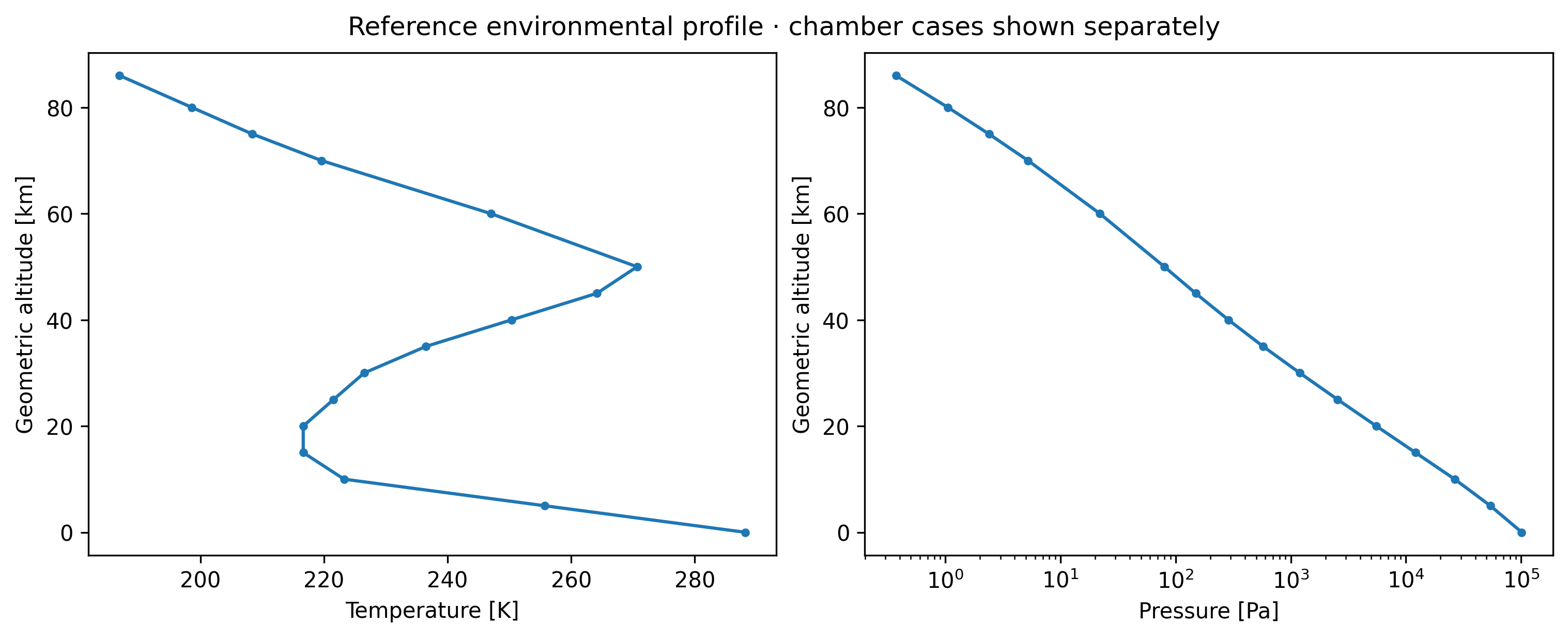
The US76 piecewise hydrostatic approximation supplies temperature and pressure over 0–86 km geometric altitude. It uses constant mean molecular mass, so its molecular-scale temperature differs from kinetic temperature by less than 0.1 K at the upper boundary. The chambers all use 288.15 K. Carrier-gas properties retain the library’s ideal-gas/transport approximations.
Python · section 1
"""Longer dry-coagulation dynamics across an ordered environmental scan."""
import matplotlib.pyplot as pltimport numpy as npfrom scripts.gpu_studies.dry_environment_sweep import (    DryEnvironmentSweep,    run_dry_sweep,)from scripts.gpu_studies.population_figures import (    describe_population,    population_figures,)
Processes, units and scope
Section titled “Processes, units and scope”Only charge-dependent Brownian coagulation operates. There is no liquid condensation, ice growth, ion source, nucleation, deposition or dilution. This avoids applying a liquid-water model at mesospheric temperatures and pressures. See the separate humidity study for water-growth dynamics near ground-level temperatures and pressures.
Dry radii are lognormal (geometric mean 35 nm, geometric standard deviation 1.6), clipped to 15–150 nm; density is 1,400 kg m⁻³. Initial charges repeat −1, 0, 0, +1 elementary charges. Active multiplicities are one. Root seed is 512. We run 2,000 steps of 0.5 s, totaling 1,000 s, at fixed box volume and environment. This longer physical window makes population and charge evolution easier to see. The density and duration differ from the humid experiment, so their raw merger totals are not directly comparable.
Every diagnostic checks each box’s material mass and net charge. Downloaded snapshots are reduced immediately to compact size/charge distributions and quantiles; individual trajectories are not published.
Python · section 2
def simulate():    """Run the complete CUDA study and return compact numerical summaries."""    report, final = run_dry_sweep(DryEnvironmentSweep())    del final    return report

def plot_results(report):    """Render saved observations without advancing the simulation."""    labels = report["labels"]    first, last = report["history"][0], report["history"][-1]    n0, n1 = np.array(first["number"]), np.array(last["number"])    loss = 100 * (n0 - n1) / n0    fig, axes = plt.subplots(1, 2, figsize=(12, 8), constrained_layout=True)    for ax, indices, title in zip(        axes,        [list(range(16)), [0, 16, 17, 18]],        [            "Reference altitude · increasing height",            "Chambers · 288.15 K · increasing pressure",        ],        strict=True,    ):        positions = np.arange(len(indices))        ax.barh(positions, loss[indices])        panel_labels = (            [labels[i] for i in indices]            if len(indices) == 16            else ["1 atm", "2 atm", "5 atm", "10 atm"]        )        ax.set_yticks(positions, panel_labels)        ax.invert_yaxis()        ax.set(title=title, xlabel="Initial particle number lost [%]")        ax.set_xlim(0, max(loss.max() * 1.15, 0.01))        ax.bar_label(ax.containers[0], fmt="%.2f", padding=3, fontsize=9)    fig.suptitle("Accepted mergers = number loss · 1,000 s")    fig, axes = plt.subplots(1, 2, figsize=(10, 4), constrained_layout=True)    altitude = report["altitude_km"]    axes[0].plot(np.array(report["temperature"])[:16], altitude, marker=".")    axes[0].set(xlabel="Temperature [K]", ylabel="Geometric altitude [km]")    axes[1].semilogx(np.array(report["pressure"])[:16], altitude, marker=".")    axes[1].set(xlabel="Pressure [Pa]", ylabel="Geometric altitude [km]")    fig.suptitle(        "Reference environmental profile · chamber cases shown separately"    )    population_figures(report, labels)    describe_population(report, labels)    print(        f"Device: {report['device']}; preparation {report['preparation_seconds']:.2f} s; "        f"synchronized stepping {report['compute_seconds']:.2f} s"    )    print("Condition | temperature [K] | pressure [Pa]")    for label, t, p in zip(        labels, report["temperature"], report["pressure"], strict=True    ):        print(f"{label} | {t:.3f} | {p:.6g}")    print(        f"At fixed 288.15 K, observed number loss is {loss[0]:.3f}% at 1 atm "        f"and {loss[-1]:.3f}% at 10 atm."    )    return report

def run_example():    """Simulate once, then render the resulting numerical summaries."""    return plot_results(simulate())
Interpret the results
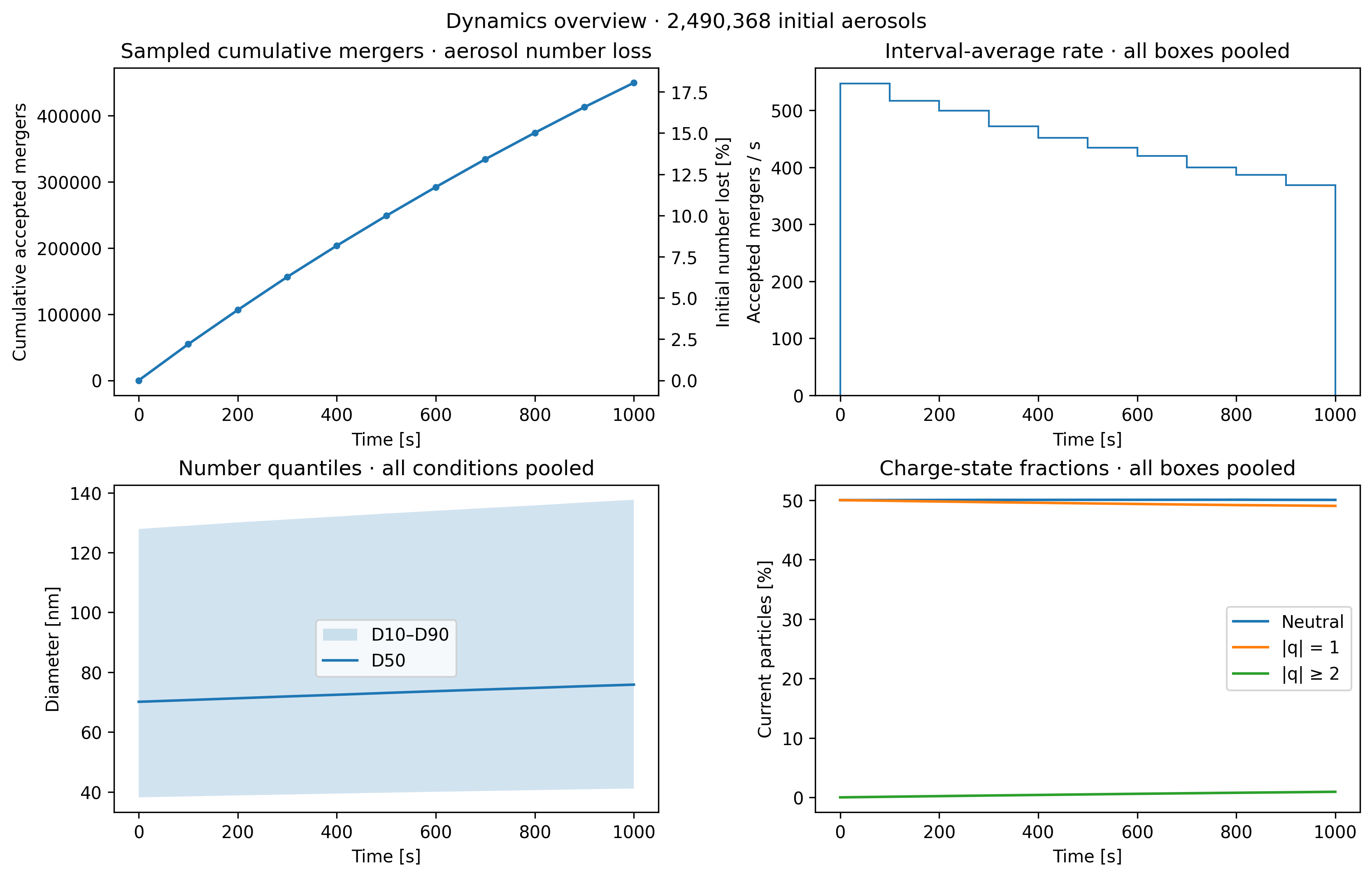
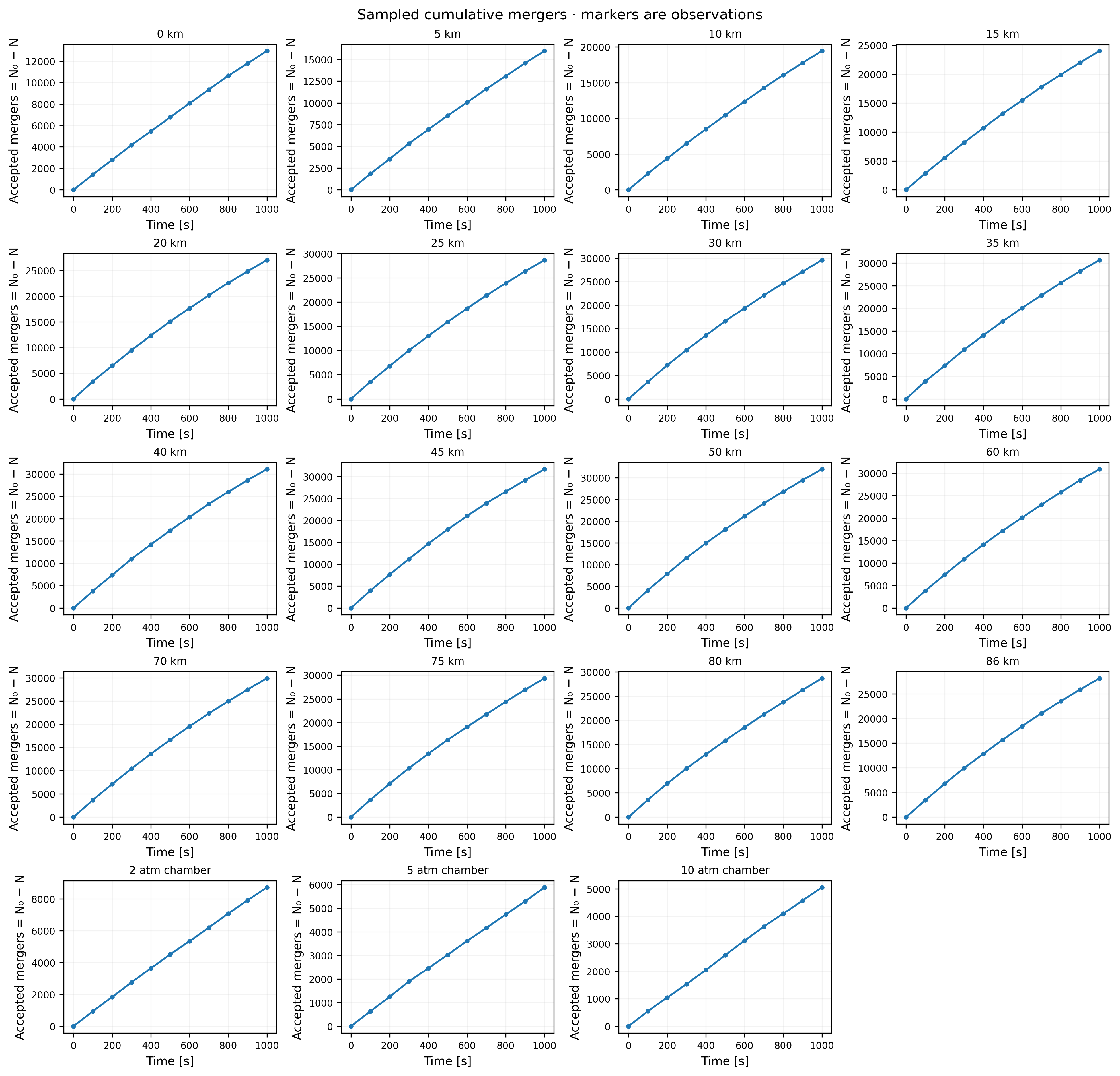
Section titled “Interpret the results”Dots on cumulative-merger curves mark saved observations. Straight connecting lines guide the eye; they do not resolve the timing of individual collisions.
Read the atmospheric and chamber comparisons separately. Altitude changes both temperature and pressure and has a nonmonotonic temperature profile. The chamber series varies pressure alone. Neither series changes aerosol number concentration initially, so changes in ambient aerosol abundance are not a cause of the displayed differences.
In this model pressure changes the carrier-gas mean free path and particle drag. At sufficiently low pressure, collision kinetics approach the free-molecular limit; lowering pressure indefinitely should not produce an unlimited collision rate. Temperature also changes thermal relative speeds and Coulomb coupling. The altitude curve can therefore have a shape that is not a simple monotonic function of height. The printed chamber comparison reports the actual observed 1-to-10-atm change without assuming its sign.
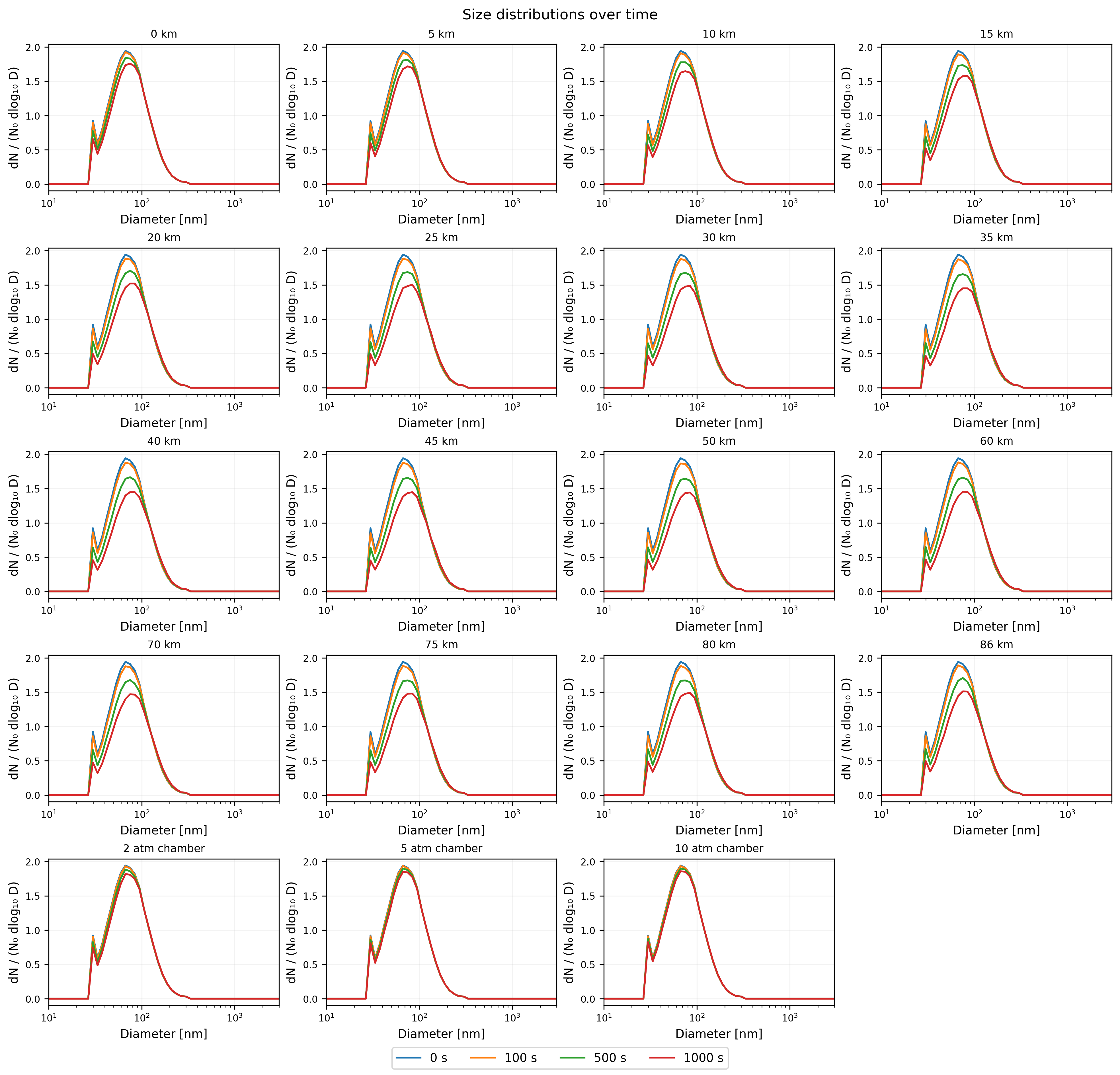
Coagulation removes particles from the count by merging them, while conserving material mass. Rightward size-spectrum motion here comes from coalescence, not vapor uptake. A growing upper tail can coexist with relatively modest median movement. Spectra use dN/(N₀ dlog₁₀D); their integrated area falls as particles merge. D10, D50 and D90 in the overview are number quantiles of all conditions pooled, not a trajectory of one representative particle.
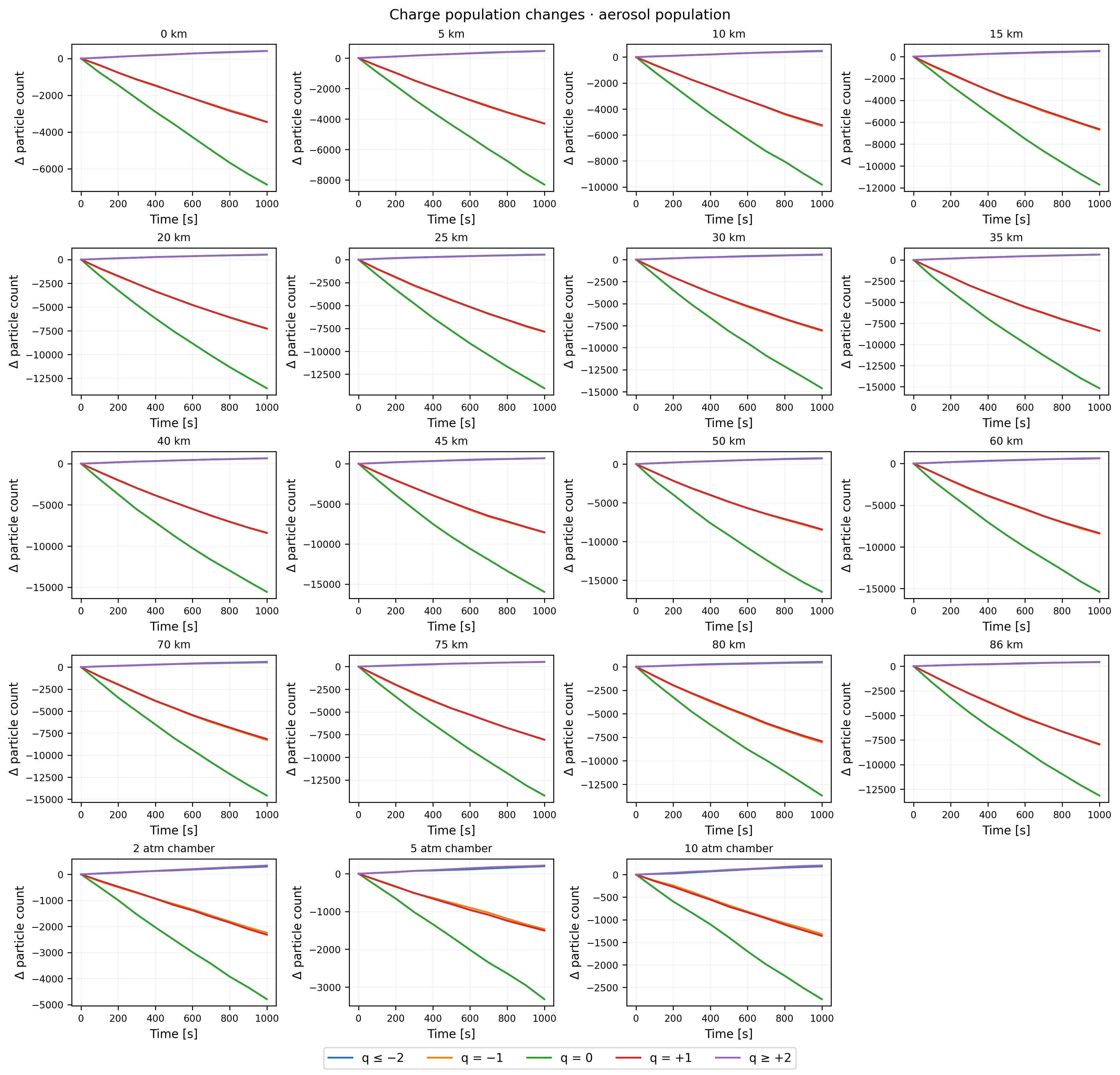
Like-sign mergers can populate higher charge states. Opposite-sign mergers can produce neutral particles. The charge-change panels show these population transfers, while the signed net charge remains exactly zero. A changing neutral fraction is compatible with exact charge conservation. Interval collision rates fluctuate because collisions are sampled stochastically and are averaged over diagnostic intervals.
The ordered bars and printed table describe one fixed-seed realization; rankings are not significance tests. The carrier-gas profile and numerical checks do not validate the assumed aerosol material, concentration, charging history or omitted processes for the real mesopause or a pressurized chamber. Timestep sensitivity is checked separately before the full-scale run.
References
Section titled “References”- U.S. Standard Atmosphere 1976, NASA-TM-X-74335: reference atmospheric layers and definitions.
- NASA/TM-2005-213659, Appendix A: piecewise hydrostatic temperature/pressure equations.
- COESA model development: molecular-scale versus kinetic temperature at the 86 km interface.
- Gopalakrishnan and Hogan (2012): transition-regime hard-sphere fit and charged collision scaling.
Python · section 3
if __name__ == "__main__": run_example()Explicit cuda invocation
result = run_example()Over 1000 s: 449,485 accepted mergers; 2,040,883 particles remain (18.04894% number loss).
Pooled number-median diameter changes from 70.121 to 75.853 nm.
Largest recorded merger count: 50 km (31,971); smallest: 10 atm chamber (5,050).
Condition | initial count | final count | mergers | final D50 [nm]
0 km | 131072 | 118128 | 12944 | 73.693
5 km | 131072 | 115113 | 15959 | 74.566
10 km | 131072 | 111647 | 19425 | 75.342
15 km | 131072 | 107083 | 23989 | 76.600
20 km | 131072 | 104042 | 27030 | 76.989
25 km | 131072 | 102438 | 28634 | 77.287
30 km | 131072 | 101498 | 29574 | 77.548
35 km | 131072 | 100422 | 30650 | 77.772
40 km | 131072 | 100003 | 31069 | 77.836
45 km | 131072 | 99385 | 31687 | 78.014
50 km | 131072 | 99101 | 31971 | 78.103
60 km | 131072 | 100166 | 30906 | 77.782
70 km | 131072 | 101198 | 29874 | 77.524
75 km | 131072 | 101746 | 29326 | 77.416
80 km | 131072 | 102394 | 28678 | 77.266
86 km | 131072 | 102939 | 28133 | 76.965
2 atm chamber | 131072 | 122360 | 8712 | 72.327
5 atm chamber | 131072 | 125198 | 5874 | 71.547
10 atm chamber | 131072 | 126022 | 5050 | 71.310
Maximum mass residual: 1.554e-15; net charge is exactly conserved in every box.
One fixed-seed realization: rankings and interval-rate fluctuations are descriptive, not significance tests.
Device: NVIDIA GeForce RTX 5060; preparation 0.81 s; synchronized stepping 3778.81 s
Condition | temperature [K] | pressure [Pa]
0 km | 288.150 | 101325
5 km | 255.676 | 54048.3
10 km | 223.252 | 26499.9
15 km | 216.650 | 12111.8
20 km | 216.650 | 5529.31
25 km | 221.552 | 2549.22
30 km | 226.509 | 1197.03
35 km | 236.513 | 574.595
40 km | 250.350 | 287.144
45 km | 264.164 | 149.101
50 km | 270.650 | 79.7791
60 km | 247.021 | 21.9587
70 km | 219.585 | 5.2209
75 km | 208.399 | 2.38814
80 km | 198.639 | 1.05247
86 km | 186.946 | 0.37338
2 atm chamber | 288.150 | 202650
5 atm chamber | 288.150 | 506625
10 atm chamber | 288.150 | 1.01325e+06
At fixed 288.15 K, observed number loss is 9.875% at 1 atm and 3.853% at 10 atm.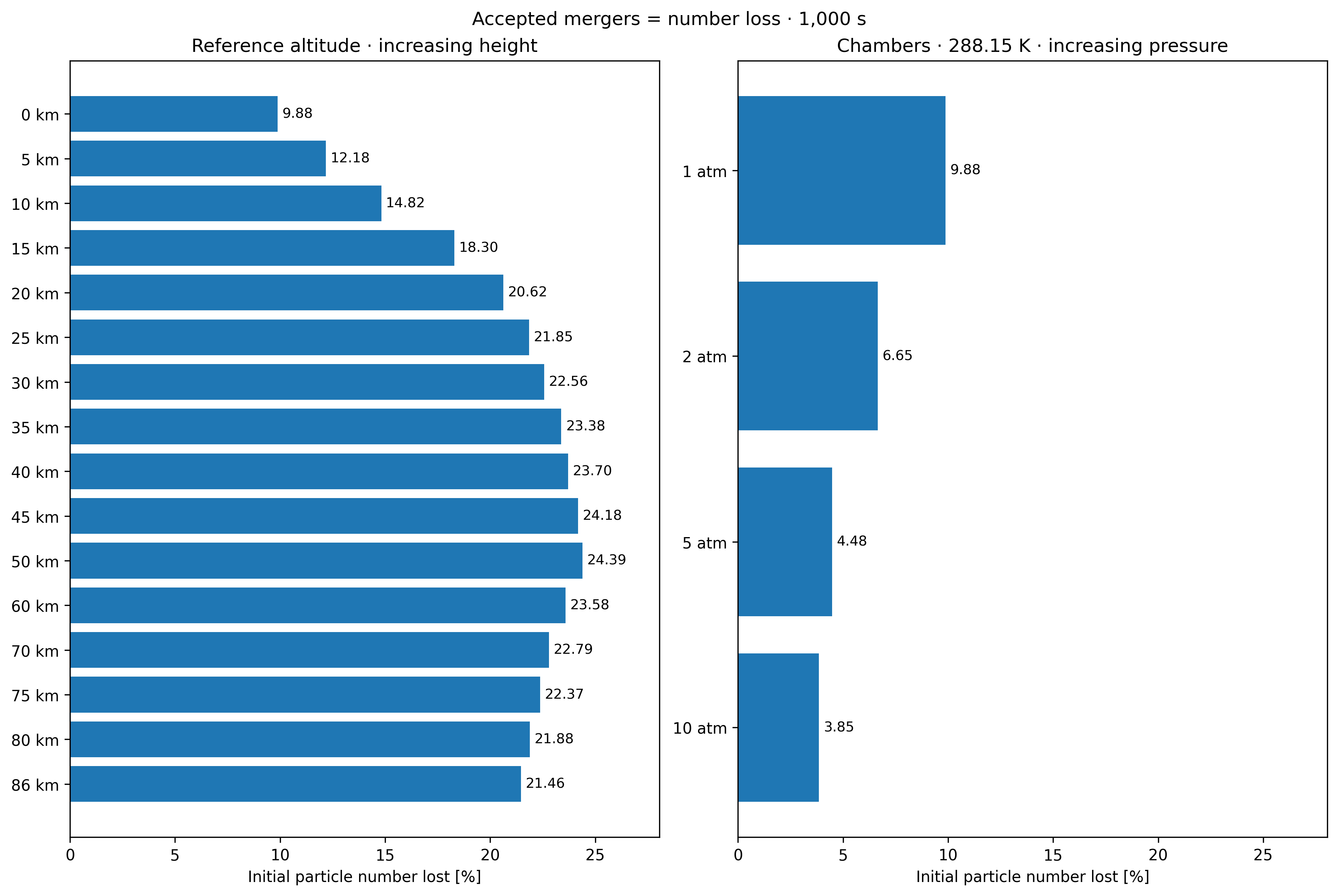
From a scan to a testable environmental hypothesis
Section titled “From a scan to a testable environmental hypothesis”The scan supports comparisons within the prescribed dry, fixed-concentration model. Mass and charge conservation explain why number loss, larger particles, and changing charge fractions can coexist. They do not establish the actual abundance or charging history at any altitude.
For a chamber question, use measured pressure and temperature, repeat seeds, and compare number decay and charge distributions against observations. For an atmospheric question, first replace the fixed concentration with an independently justified profile and quantify how that choice changes the environmental trend. Do not reuse liquid-water growth at mesospheric conditions merely because the same device can execute it; the humidity scan has a different physical domain.
Explore this topic: Atmospheric processes · GPU workflows · Charged particles and ions