

Does update ordering change a condensation calculation?
Does update ordering change a condensation calculation?
Section titled “Does update ordering change a condensation calculation?”Particles compete for a shared vapor reservoir. Updating that reservoir between particle batches changes the numerical coupling, even when all methods preserve total material. This CPU example compares three staggered update modes, then a larger-step trajectory and several batch counts.
The useful question is how to separate conservation from trajectory accuracy. Start with finite-reservoir condensation. The comparisons below provide bounded evidence for these initial conditions; they do not rank methods universally or replace a timestep-convergence study.
Python · section 1
# In Colab uncomment the following command to install particula:# Install from the repository root: `python -m pip install -e ".[extra]"`
import matplotlib.pyplot as pltimport numpy as npimport particula as parfrom particula.dynamics.condensation.species_mapping import (    CondensationSpeciesMap,)
# Set random seed for reproducibilityRANDOM_SEED = 42np.random.seed(RANDOM_SEED)
Fix the common vapor state
Section titled “Fix the common vapor state”All comparisons start from the same water concentration: 1.025 times pure-water saturation at 298.15 K and 101325 Pa. There is one condensable material, no sources or sinks, and fixed temperature. Updating gas concentration allows particles to compete for finite water; the initial saturation ratio is not maintained.
Python · section 2
# Physical constantsmolar_mass_water = 18.015e-3  # kg/mol
# Vapor pressure strategy for watervapor_pressure_water = par.gas.VaporPressureFactory().get_strategy("water_buck")
# Calculate water saturation concentrationtemperature = 298.15  # Ksaturation_concentration = vapor_pressure_water.saturation_concentration(    molar_mass=molar_mass_water, temperature=temperature)
# Supersaturated conditions (102.5% RH) to drive condensationinitial_rh = 1.025water_concentration = saturation_concentration * initial_rh
# Build gas speciesgas_species = (    par.gas.GasDataBuilder()    .set_molar_mass([molar_mass_water], "kg/mol")    .set_concentration([water_concentration], "kg/m^3")    .set_names(["H2O"])    .set_partitioning([True])    .build())
# Build atmosphereenvironment = par.gas.EnvironmentData(    temperature=[temperature],    pressure=[101325.0],    saturation_ratio=[[initial_rh]],)
print(f"Initial water concentration: {water_concentration:.6e} kg/m^3")print(f"Saturation concentration: {saturation_concentration:.6e} kg/m^3")
Initial water concentration: 2.360191e-02 kg/m^3
Saturation concentration: 2.302625e-02 kg/m^3Hold the sampled population fixed across methods
Section titled “Hold the sampled population fixed across methods”The population contains 1,000 water droplets in 1 cm³, with lognormally sampled radii around a 100 nm scale and density 1,000 kg m⁻³. Each method receives copies of the same containers, so one run cannot change the next run’s initial state. The fixed seed controls this comparison; it does not supply an ensemble error bar. Surface curvature remains part of the mass-transfer calculation.
Python · section 3
# Particle parametersdensity = 1000.0  # kg/m^3 (water droplets)volume_sim = 1e-6  # m^3 (1 cm^3)n_particles = 1000  # Moderate number for demonstration
# Generate lognormal particle distributionrng = np.random.default_rng(RANDOM_SEED)particle_radii = rng.lognormal(mean=np.log(100e-9), sigma=0.5, size=n_particles)
# Calculate particle massesparticle_masses = (4 / 3) * np.pi * particle_radii**3 * densitymass_speciation = particle_masses.reshape(-1, 1)  # Single speciesdensities = np.array([density])  # Single species density array
# Activity and surface strategiesactivity_strategy = par.particles.ActivityIdealMass()surface_strategy = par.particles.SurfaceStrategyVolume(    surface_tension=0.072, density=density)
# Build particle representationparticles = par.particles.create_resolved_particle_data(    masses=mass_speciation,    density=densities,    volume=volume_sim,)# Every strategy receives its own explicit process configuration.configuration = dict(    activity_strategy=activity_strategy,    surface_strategy=surface_strategy,    vapor_pressure_strategy=vapor_pressure_water,    species_map=CondensationSpeciesMap(("H2O",), ((0, 0),)),)
print(f"Created {n_particles} particles")print(f"Initial total particle mass: {np.sum(particle_masses):.6e} kg")print(f"Mean particle radius: {np.mean(particle_radii) * 1e9:.1f} nm")
Created 1000 particles
Initial total particle mass: 1.186594e-14 kg
Mean particle radius: 111.3 nmChange how the timestep is partitioned
Section titled “Change how the timestep is partitioned”| Mode | Split | What changes |
|---|---|---|
half |
θ = 0.5 | Equal-duration passes |
random |
θ sampled between 0 and 1 | Random division between passes |
batch |
θ = 1 | Batch updates without the second-duration contribution |
The runs below use ten batches, a 0.01 s timestep, and a shared seed. Shuffling is enabled, so equal-duration passes do not by themselves imply fixed particle ordering. Compare the printed final particle masses, then inspect the total material budget separately. No mode is designated “best” by this setup.
Python · section 4
def run_simulation(strategy, aerosol, time_step, n_steps, sub_steps=1):    """Run condensation simulation and track mass over time."""    condensation = par.dynamics.MassCondensation(condensation_strategy=strategy)
    # Copy all native containers for an independent simulation    current_aerosol = par.Aerosol(        gas=aerosol.gas.copy(),        environment=aerosol.environment.copy(),        particles=aerosol.particles.copy(),    )
    particle_mass = float(        np.sum(current_aerosol.particles.species_mass_inventory)    )    gas_mass = np.asarray(        current_aerosol.gas.concentration        * current_aerosol.particles.volume[:, None]    ).item()    mass_history = [particle_mass]    gas_mass_history = [gas_mass]
    for _step in range(n_steps):        # Execute condensation        current_aerosol = condensation.execute(            current_aerosol, time_step, sub_steps        )
        # Record masses after step        particle_mass = float(            np.sum(current_aerosol.particles.species_mass_inventory)        )        gas_mass = np.asarray(            current_aerosol.gas.concentration            * current_aerosol.particles.volume[:, None]        ).item()        mass_history.append(particle_mass)        gas_mass_history.append(gas_mass)
    combined = np.array(mass_history) + np.array(gas_mass_history)    np.testing.assert_allclose(combined, combined[0], rtol=1e-12, atol=1e-30)    return np.array(mass_history), np.array(gas_mass_history)

# Create base aerosolaerosol_base = par.Aerosol(    gas=gas_species, environment=environment, particles=particles)
# Simulation parameterstime_step = 0.01  # secondsn_steps = 100sub_steps = 1
# Run with each theta modemodes = ["half", "random", "batch"]results = {}
for mode in modes:    strategy = par.dynamics.CondensationIsothermalStaggered(        molar_mass=molar_mass_water,        **configuration,        theta_mode=mode,        num_batches=10,        shuffle_each_step=True,        random_state=RANDOM_SEED,    )    particle_mass, gas_mass = run_simulation(        strategy, aerosol_base, time_step, n_steps, sub_steps    )    results[mode] = {        "particle_mass": particle_mass,        "gas_mass": gas_mass,        "total_mass": particle_mass + gas_mass,    }    print(f"Mode '{mode}': Final particle mass = {particle_mass[-1]:.6e} kg")
Mode 'half': Final particle mass = 2.738868e-10 kgMode 'random': Final particle mass = 2.738870e-10 kgMode 'batch': Final particle mass = 2.739334e-10 kgCheck a conserved quantity, not the whole solution
Section titled “Check a conserved quantity, not the whole solution”For this single-material closed system, add extensive particle and gas masses
and evaluate rtol=1e-12 and atol=1e-30; the plotted 10⁻¹⁰ line is a visual reference,
not the assertion’s tolerance.
The saved final relative errors are near 10⁻¹⁵ for all three modes. Differences at that scale do not rank trajectory accuracy. A curve can conserve total mass while distributing it incorrectly between gas and different particle sizes.
Python · section 5
time = np.arange(n_steps + 1) * time_step
fig, (ax1, ax2) = plt.subplots(1, 2, figsize=(14, 5))
# Plot total mass over timefor mode, data in results.items():    ax1.plot(time, data["total_mass"], label=f"{mode}", linewidth=2)
ax1.set_xlabel("Time (s)")ax1.set_ylabel("Total System Mass (kg)")ax1.set_title("Total Mass Over Time")ax1.legend()ax1.ticklabel_format(style="scientific", axis="y", scilimits=(0, 0))
# Plot relative mass errorfor mode, data in results.items():    initial_mass = data["total_mass"][0]    relative_error = np.abs(data["total_mass"] - initial_mass) / initial_mass    ax2.plot(time, relative_error, label=f"{mode}", linewidth=2)
ax2.set_xlabel("Time (s)")ax2.set_ylabel("Relative Mass Error")ax2.set_title("Mass Conservation Error")ax2.set_yscale("log")ax2.legend()ax2.axhline(    y=1e-10, color="gray", linestyle="--", alpha=0.5, label="Target (1e-10)")
plt.tight_layout()plt.show()
# Print final relative errorsprint("\nFinal Relative Mass Errors:")for mode, data in results.items():    initial_mass = data["total_mass"][0]    final_error = np.abs(data["total_mass"][-1] - initial_mass) / initial_mass    print(f"  {mode}: {final_error:.2e}")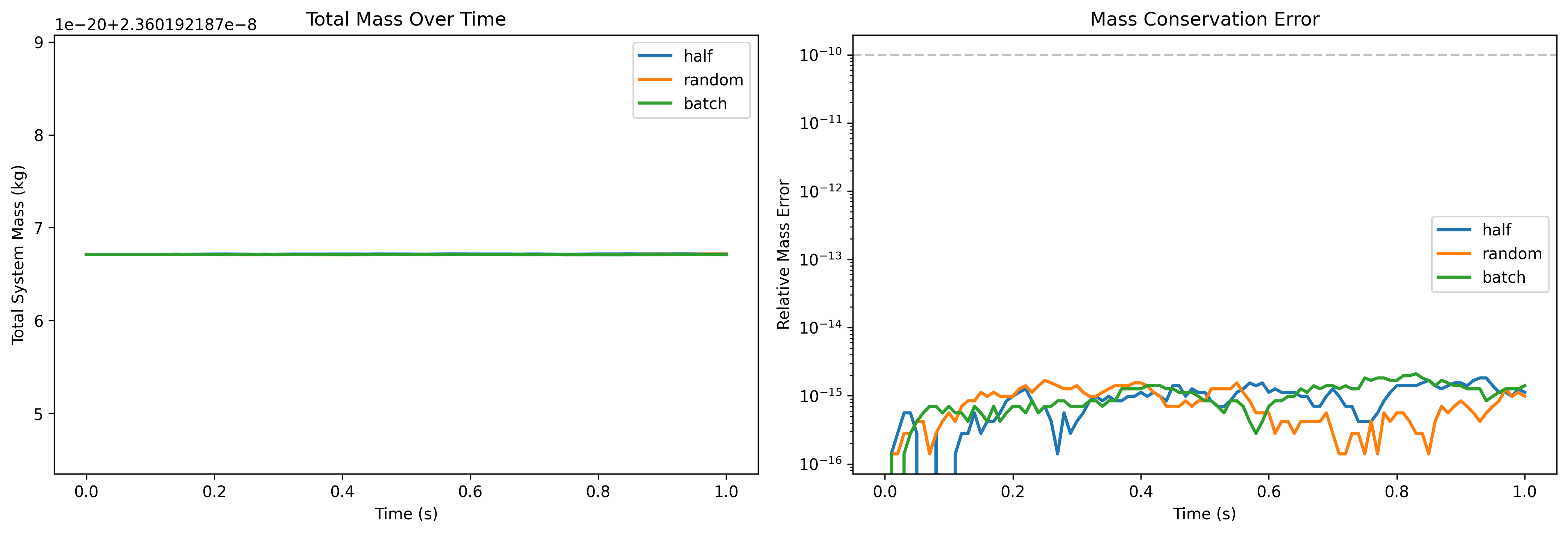
Final Relative Mass Errors:
  half: 1.12e-15
  random: 9.81e-16
  batch: 1.40e-15
Compare a larger timestep under the same initial conditions
Section titled “Compare a larger timestep under the same initial conditions”The next experiment uses 0.1 s steps for 5 s and compares random staggered updates with simultaneous updates. Read particle mass and total-mass error as separate diagnostics. Both histories remain finite in this saved calculation; that observation neither demonstrates instability of the simultaneous method nor guarantees stability for another particle loading or timestep.
Python · section 6
# Larger time step for the bounded comparisonlarge_time_step = 0.1  # 10x largern_steps_stability = 50
# Staggered strategystaggered_strategy = par.dynamics.CondensationIsothermalStaggered(    molar_mass=molar_mass_water,    **configuration,    theta_mode="random",    num_batches=10,    random_state=RANDOM_SEED,)
# Simultaneous strategysimultaneous_strategy = par.dynamics.CondensationIsothermal(    molar_mass=molar_mass_water,    **configuration,    diffusion_coefficient=2e-5,    accommodation_coefficient=1.0,    update_gases=True,)
# Run both strategiesstaggered_mass, staggered_gas = run_simulation(    staggered_strategy, aerosol_base, large_time_step, n_steps_stability)simultaneous_mass, simultaneous_gas = run_simulation(    simultaneous_strategy, aerosol_base, large_time_step, n_steps_stability)
# Plot comparisontime_stability = np.arange(n_steps_stability + 1) * large_time_step
fig, (ax1, ax2) = plt.subplots(1, 2, figsize=(14, 5))
# Particle mass evolutionax1.plot(    time_stability, staggered_mass, label="Staggered (random)", linewidth=2)ax1.plot(    time_stability,    simultaneous_mass,    label="Simultaneous",    linewidth=2,    linestyle="--",)ax1.set_xlabel("Time (s)")ax1.set_ylabel("Particle Mass (kg)")ax1.set_title(f"Particle Mass (dt = {large_time_step}s)")ax1.legend()
# Mass conservation comparisonstaggered_total = staggered_mass + staggered_gassimultaneous_total = simultaneous_mass + simultaneous_gas
staggered_error = (    np.abs(staggered_total - staggered_total[0]) / staggered_total[0])simultaneous_error = (    np.abs(simultaneous_total - simultaneous_total[0]) / simultaneous_total[0])
ax2.plot(time_stability, staggered_error, label="Staggered", linewidth=2)ax2.plot(    time_stability,    simultaneous_error,    label="Simultaneous",    linewidth=2,    linestyle="--",)ax2.set_xlabel("Time (s)")ax2.set_ylabel("Relative Mass Error")ax2.set_title("Mass Conservation at Large Time Steps")ax2.set_yscale("log")ax2.legend()
plt.tight_layout()plt.show()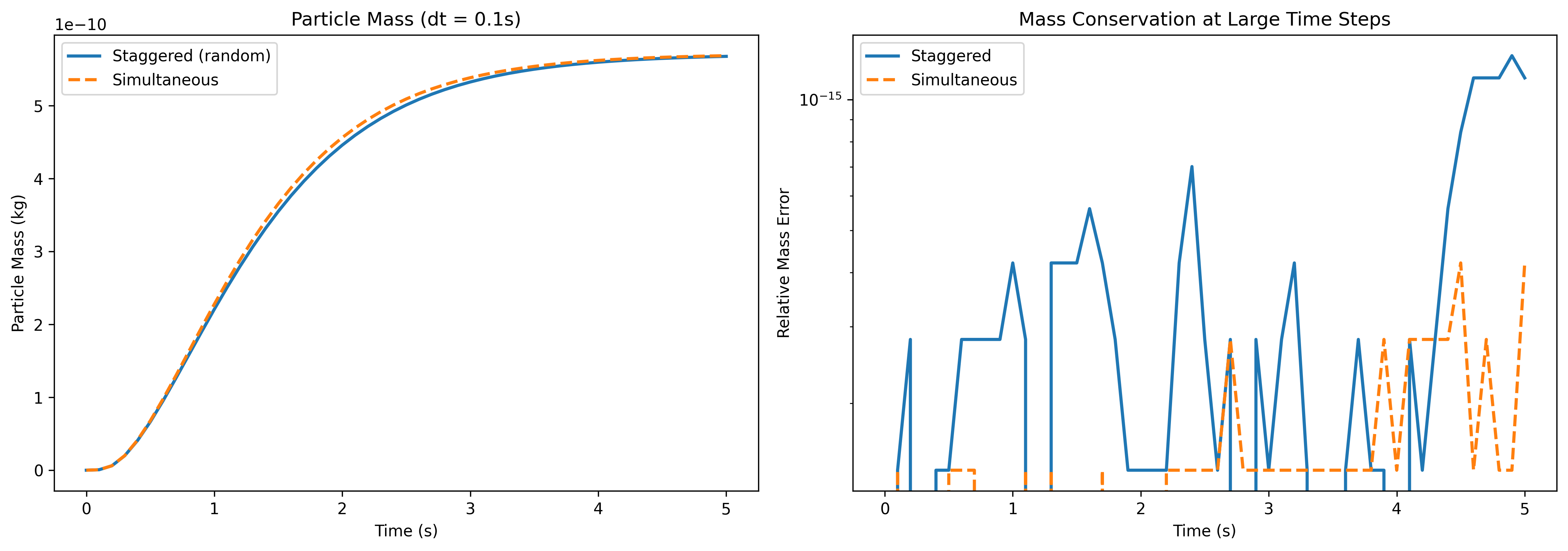
Treat batch count as a numerical choice to investigate
Section titled “Treat batch count as a numerical choice to investigate”One, five, ten, and twenty batches change how frequently gas feedback is applied. The final plot reports total-mass error only. It does not measure execution cost, particle-size error, or convergence toward a reference solution, so it cannot justify a particle-count-based recommendation for batch number.
To choose a batch count for a study, compare gas concentration and size-resolved mass transfer against a sufficiently refined timestep, then measure cost for the intended population. Keep initial conditions and random-stream policy consistent across those comparisons.
Python · section 7
# Demonstrate effect of num_batchesbatch_counts = [1, 5, 10, 20]batch_results = {}
for num_batches in batch_counts:    strategy = par.dynamics.CondensationIsothermalStaggered(        molar_mass=molar_mass_water,        **configuration,        theta_mode="half",        num_batches=num_batches,        random_state=RANDOM_SEED,    )    particle_mass, gas_mass = run_simulation(        strategy, aerosol_base, time_step, n_steps    )    batch_results[num_batches] = particle_mass + gas_mass
# Plot mass conservation vs batch countfig, ax = plt.subplots(figsize=(8, 5))
for num_batches, total_mass in batch_results.items():    initial = total_mass[0]    error = np.abs(total_mass - initial) / initial    ax.plot(time, error, label=f"num_batches={num_batches}", linewidth=2)
ax.set_xlabel("Time (s)")ax.set_ylabel("Relative Mass Error")ax.set_title("Effect of Batch Count on Mass Conservation")ax.set_yscale("log")ax.legend()plt.tight_layout()plt.show()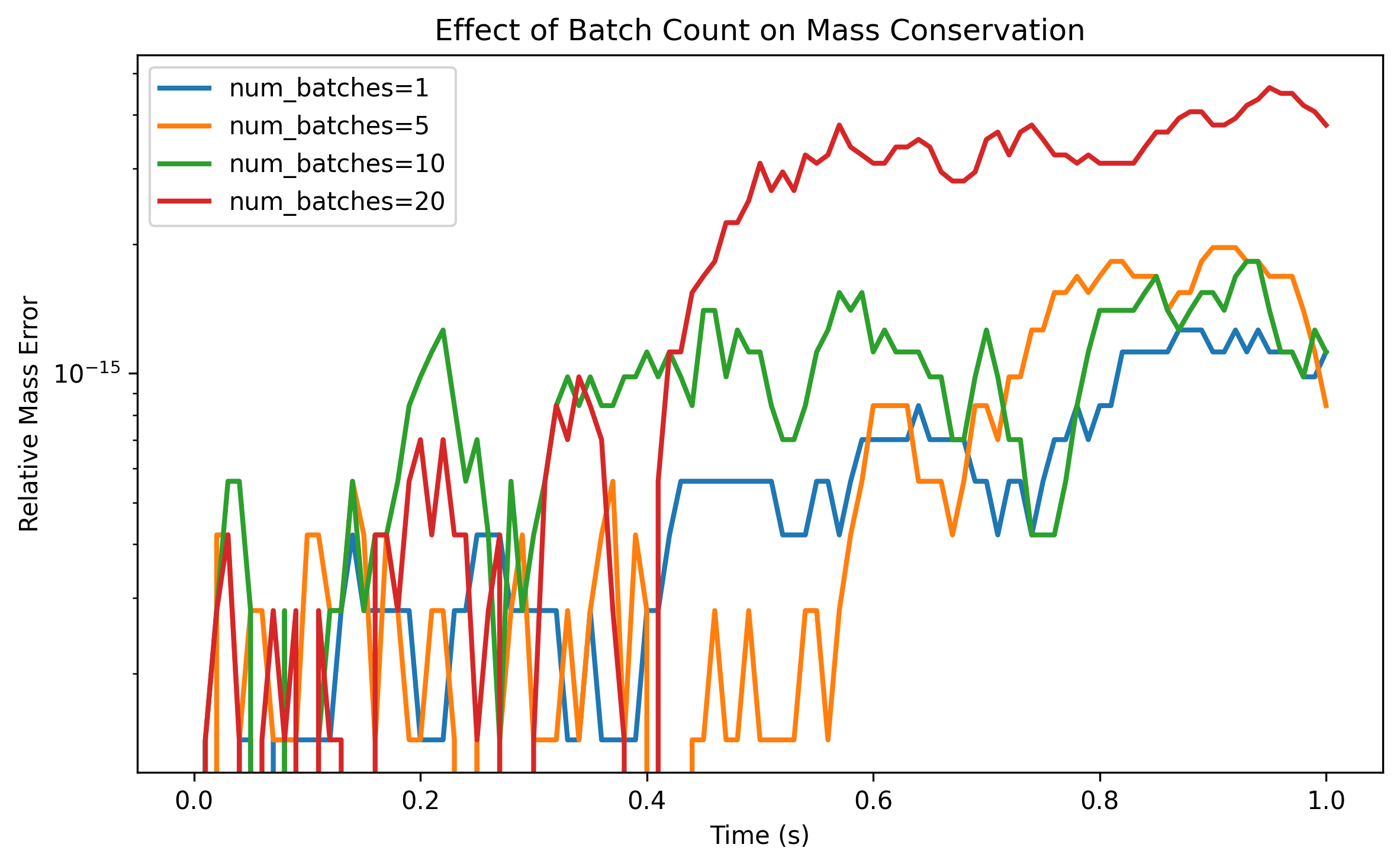
Design the next numerical experiment
Section titled “Design the next numerical experiment”The displayed runs conserve the combined water inventory, yet update ordering and batch count remain separate numerical choices. Conservation is necessary for this closed system but is not enough to select an accurate trajectory.
A useful extension is a timestep ladder for each mode, comparing final vapor, particle-mass quantiles, and the time of a defined growth event. Repeat seeded runs where random ordering matters and report both sensitivity and runtime. Only then select settings for a scientific question. See the condensation strategy guide for supported behavior and the numerical-methods topic for connections to other validation examples.
Explore this topic: Numerical methods