

Compare coagulation after matching distribution units
Python · section 1
"""Compare PMF and PDF coagulation representations.
Builds PMF and PDF aerosols over a shared radius grid, configures Browniancoagulation with both ``distribution_type="discrete"`` and``distribution_type="continuous_pdf"``, runs short guarded steps, convertsbetween representations via ``get_pdf_distribution_in_pmf``, and plotsbefore/after concentrations in PMF and PDF units for side-by-side behaviorchecks. Uses modest grids and a single short step to keep runtime quick.
Example:    Execute the script to see matching PMF and PDF concentration curves    before and after coagulation, enabling comparison across    representations."""
'Compare PMF and PDF coagulation representations.\n\nBuilds PMF and PDF aerosols over a shared radius grid, configures Brownian\ncoagulation with both ``distribution_type="discrete"`` and\n``distribution_type="continuous_pdf"``, runs short guarded steps, converts\nbetween representations via ``get_pdf_distribution_in_pmf``, and plots\nbefore/after concentrations in PMF and PDF units for side-by-side behavior\nchecks. Uses modest grids and a single short step to keep runtime quick.\n\nExample:\n Execute the script to see matching PMF and PDF concentration curves\n before and after coagulation, enabling comparison across\n representations.\n'Compare coagulation after matching distribution units
Section titled “Compare coagulation after matching distribution units”Would two solvers disagree, or are their curves simply expressed in different measures? This example evolves a PMF and a PDF with the same Brownian mechanism, then converts each into the other’s plotting units. You will learn to separate a coordinate/measure difference from a numerical evolution difference.
Start with PMF evolution, PDF evolution, or the distribution conversion example.
Python · section 2
# In Colab uncomment the following command to install particula:# Install from the repository root: `python -m pip install -e ".[extra]"`import matplotlib.pyplot as pltimport numpy as npimport particula as parfrom scipy.integrate import trapezoidMatch the physical inputs
Section titled “Match the physical inputs”Both populations use 150 radius nodes over 10 nm–10 µm, a 120 nm lognormal radius scale, geometric standard deviation 1.5, and target number density 10¹⁰ m⁻³. Density is 1000 kg m⁻³, temperature 298.15 K, and pressure 101325 Pa. The PMF stores m⁻³ per bin; the PDF stores m⁻⁴ per radius. Separate container copies keep advancing one population from changing the other.
Python · section 3
# Shared grid (modest resolution)radius_bins = np.logspace(-8, -5, 150)  # m (10 nm to 10 um)
# Lognormal parameters (kept small for speed)mode = np.array([120e-9])gsd = np.array([1.5])number_conc = np.array([1e10])  # m^-3 total
# PMF (number per bin)concentration_pmf = par.particles.get_lognormal_pmf_distribution(    x_values=radius_bins,    mode=mode,    geometric_standard_deviation=gsd,    number_of_particles=number_conc,)
# PDF (number per size)concentration_pdf = par.particles.get_lognormal_pdf_distribution(    x_values=radius_bins,    mode=mode,    geometric_standard_deviation=gsd,    number_of_particles=number_conc,)
# Native ambient environment. GasData requires a species axis, so a# zero-concentration, non-partitioning carrier fills that axis. Coagulation# does not consume it; ambient pressure is specified independently.environment = par.gas.EnvironmentData(    temperature=np.array([298.15]),    pressure=np.array([101325.0]),    saturation_ratio=np.zeros((1, 1)),)gas = par.gas.GasData(    name=["carrier"],    molar_mass=np.array([0.02897]),    partitioning=np.array([False]),    concentration=np.zeros((1, 1)),)
# PMF particlesparticles_pmf = par.particles.create_particle_data_from_radii(    radii=radius_bins,    concentration=concentration_pmf,    distribution_type="discrete",    density=1000.0,)
aerosol_pmf = par.Aerosol(    particles=particles_pmf, gas=gas.copy(), environment=environment.copy())
# PDF particlesparticles_pdf = par.particles.create_particle_data_from_radii(    radii=radius_bins,    concentration=concentration_pdf,    distribution_type="continuous_pdf",    density=1000.0,)
aerosol_pdf = par.Aerosol(    particles=particles_pdf, gas=gas.copy(), environment=environment.copy())
Hold the mechanism fixed
Section titled “Hold the mechanism fixed”Both wrappers use Brownian coagulation, selecting discrete or continuous_pdf
to match storage. There are no gas-phase transfers or external particle losses.
Changing this setting alone is not a conversion of an existing concentration
array; the initial arrays were constructed in their respective measures.
Python · section 4
coagulation_pmf = par.dynamics.Coagulation(    coagulation_strategy=(        par.dynamics.BrownianCoagulationBuilder()        .set_distribution_type("discrete")        .build()    ))
coagulation_pdf = par.dynamics.Coagulation(    coagulation_strategy=(        par.dynamics.BrownianCoagulationBuilder()        .set_distribution_type("continuous_pdf")        .build()    ))
print(coagulation_pmf)print(coagulation_pdf)
<particula.dynamics.particle_process.Coagulation object at 0x7f23516107d0>
<particula.dynamics.particle_process.Coagulation object at 0x7f23521cbb30>Compare the same elapsed time
Section titled “Compare the same elapsed time”Each population advances one hour using 100 substeps. Copies of concentration before and after preserve the comparison even though execution mutates the aerosol. Agreement in these snapshots would still require a refinement study before it could establish accuracy.
Python · section 5
time_step = 3600  # seconds (1 hour)sub_steps = 100
# PMF runpmf_before = aerosol_pmf.particles.concentration[0].copy()aerosol_pmf_after = coagulation_pmf.execute(    aerosol_pmf, time_step=time_step, sub_steps=sub_steps)pmf_after = aerosol_pmf_after.particles.concentration[0].copy()
# PDF runpdf_before = aerosol_pdf.particles.concentration[0].copy()aerosol_pdf_after = coagulation_pdf.execute(    aerosol_pdf, time_step=time_step, sub_steps=sub_steps)pdf_after = aerosol_pdf_after.particles.concentration[0].copy()
Put both results in common units
Section titled “Put both results in common units”The conversion uses radius-dependent bin widths, so it changes curve shape as well as magnitude on this logarithmically spaced grid. The printed initial totals compare a PMF sum with a trapezoidal PDF integral. Finite-grid quadrature and conversion conventions can leave small differences; neither operation is an independent physical benchmark.
Python · section 6
pdf_as_pmf_before = par.particles.get_pdf_distribution_in_pmf(    x_array=radius_bins, distribution=pdf_before, to_pdf=False)pdf_as_pmf_after = par.particles.get_pdf_distribution_in_pmf(    x_array=radius_bins, distribution=pdf_after, to_pdf=False)
pmf_as_pdf_before = par.particles.get_pdf_distribution_in_pmf(    x_array=radius_bins, distribution=pmf_before, to_pdf=True)pmf_as_pdf_after = par.particles.get_pdf_distribution_in_pmf(    x_array=radius_bins, distribution=pmf_after, to_pdf=True)
# Quick consistency checknumber_pmf = pmf_before.sum()number_pdf = trapezoid(pdf_before, x=radius_bins)print(f"Total number PMF: {number_pmf:.2e} m^-3")print(f"Total number PDF: {number_pdf:.2e} m^-3 (integrated)")
Total number PMF: 1.00e+10 m^-3
Total number PDF: 1.00e+10 m^-3 (integrated)Read the two overlays as one comparison
Section titled “Read the two overlays as one comparison”The first figure expresses both populations in number per volume per bin; the second expresses both per unit radius. Compare corresponding before curves to assess initialization and conversion, then corresponding after curves to assess evolution. Do not compare raw peak heights between the two figures: their units differ. A visual overlay can conceal small integrated mass or number errors.
Python · section 7
fig, ax = plt.subplots(figsize=(8, 5))ax.plot(radius_bins, pmf_before, label="PMF before", color="tab:blue")ax.plot(radius_bins, pmf_after, label="PMF after", color="tab:orange")ax.plot( radius_bins, pdf_as_pmf_before, label="PDF→PMF before", color="tab:green", linestyle="--",)ax.plot( radius_bins, pdf_as_pmf_after, label="PDF→PMF after", color="tab:red", linestyle="--",)ax.set_xscale("log")ax.set_xlim(1e-8, 1e-5)ax.set_xlabel("Particle radius (m)")ax.set_ylabel(r"Number concentration ($m^{-3}$)")ax.set_title("PMF vs PDF coagulation (converted to PMF units)")ax.legend()ax.grid(alpha=0.3)plt.show()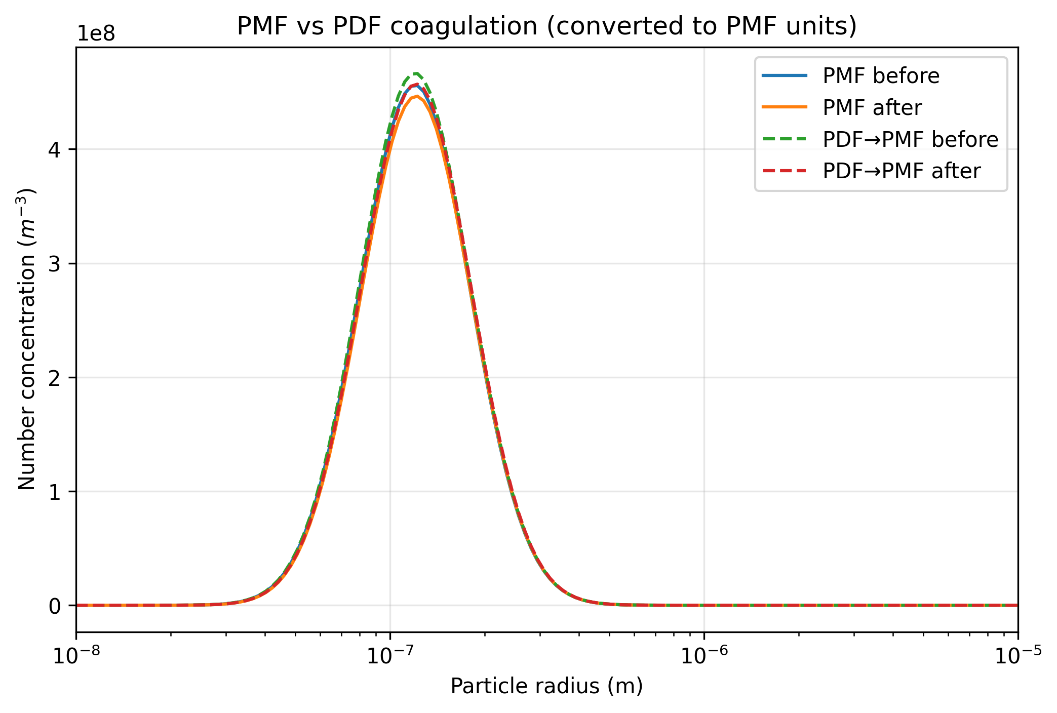
Python · section 8
fig, ax = plt.subplots(figsize=(8, 5))ax.plot( radius_bins, pmf_as_pdf_before, label="PMF→PDF before", color="tab:blue")ax.plot( radius_bins, pmf_as_pdf_after, label="PMF→PDF after", color="tab:orange")ax.plot( radius_bins, pdf_before, label="PDF before", color="tab:green", linestyle="--",)ax.plot( radius_bins, pdf_after, label="PDF after", color="tab:red", linestyle="--")ax.set_xscale("log")ax.set_xlim(1e-8, 1e-5)ax.set_xlabel("Particle radius (m)")ax.set_ylabel(r"PDF concentration ($m^{-4}$)")ax.set_title("PMF vs PDF coagulation (PDF units)")ax.legend()ax.grid(alpha=0.3)plt.show()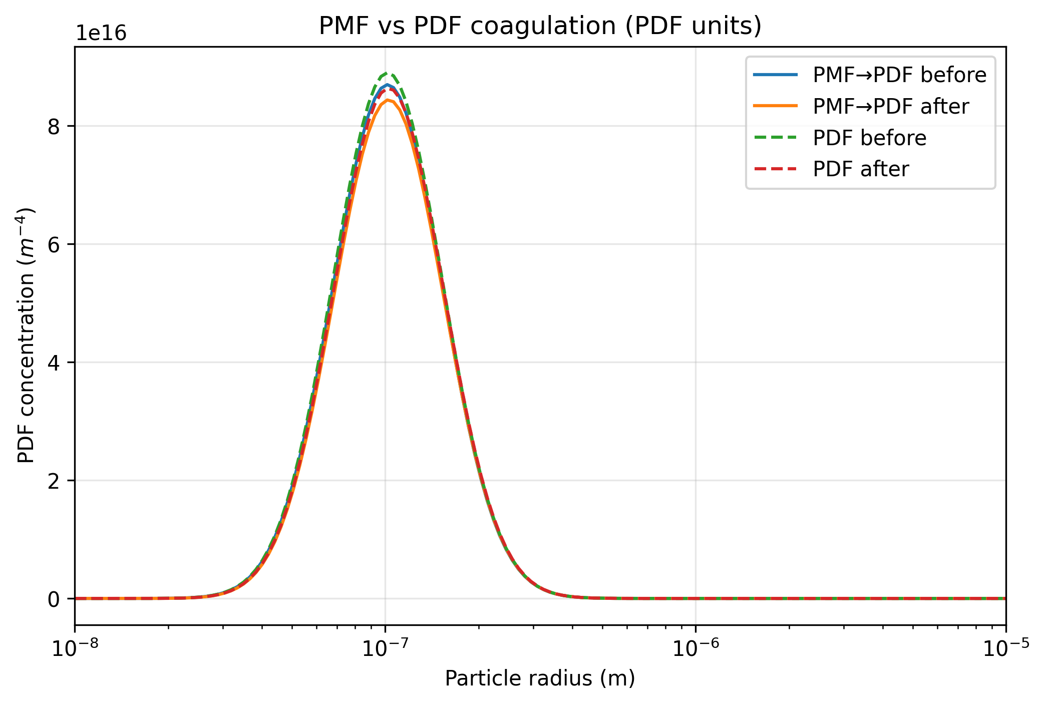
Identify what this comparison cannot settle
Section titled “Identify what this comparison cannot settle”Native construction retains the declared input arrays. Neither finite-grid method is guaranteed exactly mass conservative, and this run does not vary grid extent, resolution, or timestep. Similar-looking spectra are evidence for this workload, not proof of solver equivalence.
Turn an overlay into an error study
Section titled “Turn an overlay into an error study”Matching measures makes a scientific comparison possible; it does not complete one. Refine the grid and substeps separately, report integrated number and mass, and compare against an independent limiting-case solution when available.
The time-evolution example adds a particle-resolved population and follows a common diagnostic through time. That is a useful starting point for asking whether a research conclusion depends on representation rather than on plotting convention.
Explore this topic: Comparing representations