

A compact particle-resolved collision calculation
A compact particle-resolved collision calculation
Section titled “A compact particle-resolved collision calculation”How do you check that merging particles preserves their material? This example uses a sampled population, advances Brownian coagulation for 200 s, and checks the surviving count-weighted mass. It introduces the bookkeeping needed for later composition-resolved studies.
Start with represented counts and volume. For a longer trajectory and a larger sample, see the particle-resolved pattern.
Python · section 1
# In Colab uncomment the following command to install particula:# Install from the repository root: `python -m pip install -e ".[extra]"`import matplotlib.pyplot as pltimport numpy as npimport particula as parSeparate sampling weights from physical abundance
Section titled “Separate sampling weights from physical abundance”The 12,000 samples use lognormal radius scales of 80 and 200 nm, geometric standard deviations 1.4 and 1.5, and relative weights 4000:2000. Those weights set the mixture, not the final physical number density. Unit represented counts in 10⁻³ m³ give 1.2×10⁷ m⁻³. Spherical masses use 1000 kg m⁻³.
Temperature and pressure are fixed at 298.15 K and 101325 Pa. The initial sampling seed selects one realization; it does not quantify stochastic uncertainty in the collision process.
Python · section 2
# Sample radii (small sample for speed)np.random.seed(42)radii_sample = par.particles.get_lognormal_sample_distribution(    mode=np.array([80e-9, 200e-9]),    geometric_standard_deviation=np.array([1.4, 1.5]),    number_of_particles=np.array([4e3, 2e3]),    number_of_samples=12_000,)
# Mass from radius assuming 1 g/cm^3density = np.array([1_000.0])mass_sample = 4 / 3 * np.pi * radii_sample**3 * density
# Native ambient environment. GasData requires a species axis, so a# zero-concentration, non-partitioning carrier fills that axis. Coagulation# does not consume it; ambient pressure is specified independently.environment = par.gas.EnvironmentData(    temperature=np.array([298.15]),    pressure=np.array([101325.0]),    saturation_ratio=np.zeros((1, 1)),)gas = par.gas.GasData(    name=["carrier"],    molar_mass=np.array([0.02897]),    partitioning=np.array([False]),    concentration=np.zeros((1, 1)),)
# Particle-resolved representationparticles_resolved = par.particles.create_resolved_particle_data(    masses=mass_sample,    density=density,    volume=1e-3,)
aerosol_resolved = par.Aerosol(    particles=particles_resolved, gas=gas, environment=environment)
Choose individual-particle collision bookkeeping
Section titled “Choose individual-particle collision bookkeeping”The Brownian strategy’s particle_resolved setting matches the sampled
container. There are no gas transfers or external sources, so the sum of
represented material should remain unchanged as collision partners merge.
Python · section 3
coagulation_strategy = (    par.dynamics.BrownianCoagulationBuilder()    .set_distribution_type("particle_resolved")    .build())coagulation_process = par.dynamics.Coagulation(    coagulation_strategy=coagulation_strategy)
print(coagulation_process)
<particula.dynamics.particle_process.Coagulation object at 0x7f03b7e1cce0>Check surviving material, not array length
Section titled “Check surviving material, not array length”Execution advances 200 s in five substeps. The assertion sums each surviving slot’s mass times its represented count and compares with the initial mass. It then filters inactive slots for plotting. Storage capacity can remain fixed even when the physical particle count falls.
Python · section 4
time_step = 200  # secondssub_steps = 5
radii_before = aerosol_resolved.particles.radii[0].copy()initial_mass = np.sum(mass_sample)
_aerosol_after = coagulation_process.execute(    aerosol_resolved, time_step=time_step, sub_steps=sub_steps)radii_after = _aerosol_after.particles.radii[0].copy()np.testing.assert_allclose(    np.sum(        _aerosol_after.particles.masses        * _aerosol_after.particles.concentration[..., None]    ),    initial_mass,    rtol=1e-12,    atol=1e-30,)radii_after = radii_after[_aerosol_after.particles.concentration[0] > 0]
Interpret the normalized histogram cautiously
Section titled “Interpret the normalized histogram cautiously”density=True makes each histogram a probability density per metre of radius,
with independent area normalization. It cannot show total particle-number loss.
The displayed range is set by initial extrema; any grown particles beyond it
would also be absent from this display. A number-per-volume histogram with an
expanded range is a better diagnostic for a quantitative abundance study.
Python · section 5
bins = np.logspace(    np.log10(radii_before.min()), np.log10(radii_before.max()), 80).tolist()
fig, ax = plt.subplots(figsize=(8, 5))ax.hist(    radii_before,    bins=bins,    histtype="step",    color="tab:blue",    label="Before",    density=True,)ax.hist(    radii_after,    bins=bins,    histtype="step",    color="tab:orange",    label="After",    density=True,)ax.set_xscale("log")ax.set_xlabel("Particle radius (m)")ax.set_ylabel("Active-particle probability density (m$^{-1}$)")ax.set_title("Particle-resolved coagulation (Brownian)")ax.legend()ax.grid(alpha=0.3)plt.show()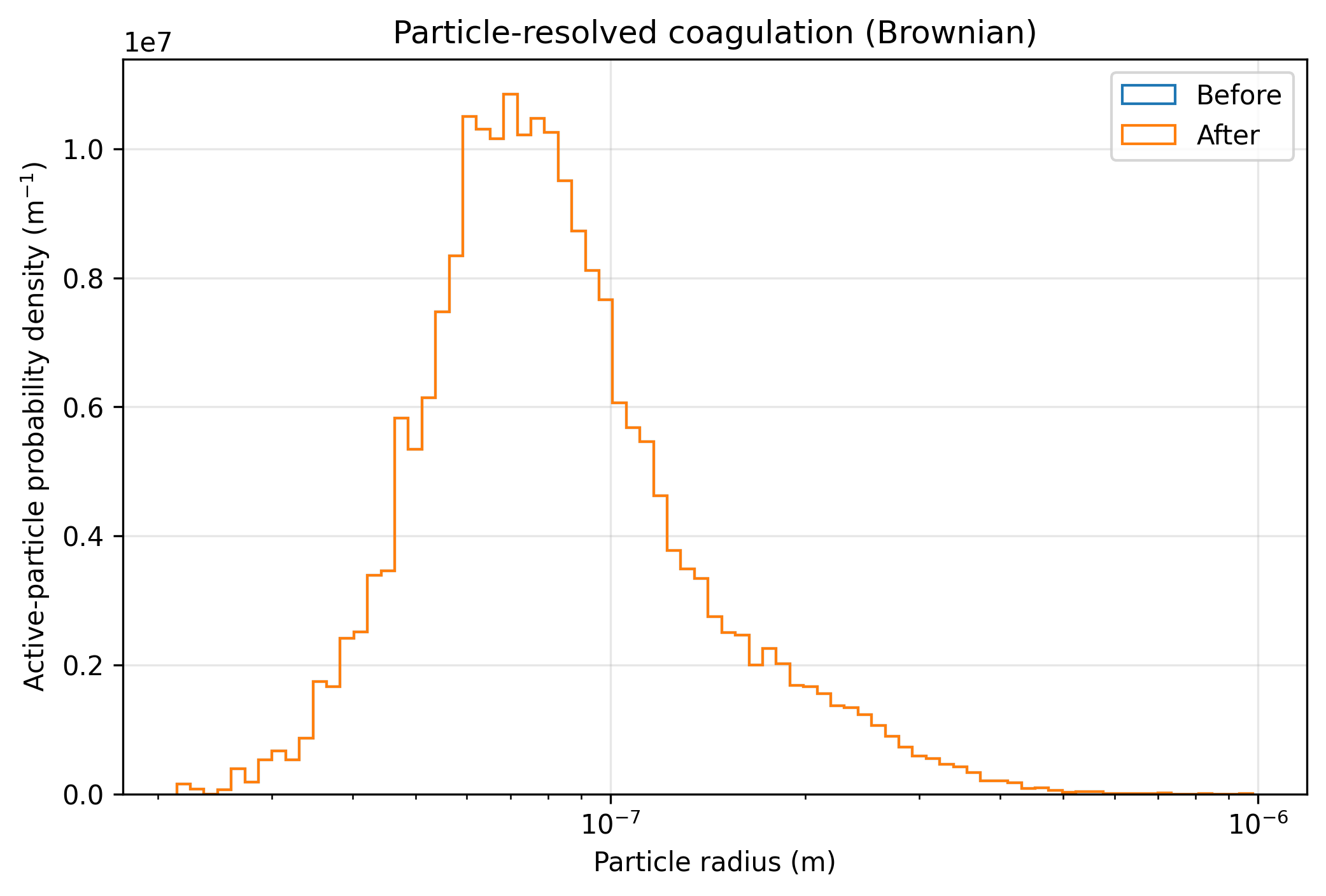
Carry the inventory check into a research model
Section titled “Carry the inventory check into a research model”The calculation establishes an execution path with an explicit material check. A small histogram change at this low abundance and short time is compatible with a small collision effect, but it is not a convergence or sensitivity study.
To study how mixing state develops, add separate material lanes for two initial populations and track composition conditional on radius. Check each material’s inventory, count the collision-driven number loss, and repeat seeds while refining substeps. The matched time comparison provides a route to comparing aggregate behavior across representations.
Explore this topic: Particle-resolved populations