

Aerosol size distributions
One population, different size spectra
Section titled “One population, different size spectra”Why can two plots of the same aerosol population have different heights and shapes? The ordinate may describe number per unit diameter, number in a bin, or number per logarithmic interval. Recognizing that distinction is essential when comparing an instrument spectrum with a model’s initial conditions.
Here we construct one- and two-component lognormal populations, compare a diameter density with bin-integrated numbers, and convert the density into Particula’s native radius coordinate. The calculation uses CPU NumPy arrays; familiarity with native particle construction helps with the last step. The populations are illustrative, not fitted measurements.
Python · section 1
# In Colab uncomment the following command to install particula:# Install from the repository root: `python -m pip install -e ".[extra]"`import matplotlib.pyplot as pltimport numpy as npimport particula as parA density needs a coordinate
Section titled “A density needs a coordinate”For diameter
Here mode, but the helper passes
it to SciPy as scale: it is
The helper normalizes each component numerically over the supplied grid to its
requested total
For the first plots,
Choose the size range
Section titled “Choose the size range”Logarithmic spacing resolves several size decades with a manageable grid. The domain below is 0.001–10 µm in diameter. Logarithmic spacing of the points does not itself turn a density per diameter into a density per log diameter.
Python · section 2
# Define the x_values as a range of particle diametersx_values = np.logspace(-3, 1, 2000) # From 0.001 to 10 micronsStart with one component
Section titled “Start with one component”The first component has a geometric mean diameter of 0.02 µm, geometric standard deviation 1.4, and total number 1,000. Keeping the total separate from size and spread lets us distinguish abundance from distribution shape.
Python · section 4
# Single mode distributionsingle_mode_gsd = np.array([1.4])single_mode = np.array([0.02])single_mode_nparticles = np.array([1e3])
single_mode_distribution = par.particles.get_lognormal_pdf_distribution(    x_values, single_mode, single_mode_gsd, single_mode_nparticles)
Add a second component
Section titled “Add a second component”The second population retains the first component and adds a broader one centered at 1 µm, also with total number 1,000. Equal component totals do not imply equal peak heights in a density per unit diameter.
Python · section 6
# Multi-mode distributionmulti_mode_gsd = np.array([1.4, 1.8])multi_mode = np.array([0.02, 1.0])multi_mode_nparticles = np.array([1e3, 1e3])
multi_mode_distribution = par.particles.get_lognormal_pdf_distribution(    x_values, multi_mode, multi_mode_gsd, multi_mode_nparticles)
Compare densities per diameter
Section titled “Compare densities per diameter”The next plot uses a logarithmic horizontal axis but retains
Python · section 8
plt.figure(figsize=(10, 6))plt.plot(x_values, single_mode_distribution, label="Single Mode", linewidth=4)plt.plot(x_values, multi_mode_distribution, label="Multi Mode")plt.title("Lognormal Particle Size Distribution")plt.xlabel("Particle Diameter (μm)")plt.ylabel("Number per micrometre of diameter")plt.xscale("log")plt.legend()plt.grid(True)plt.show()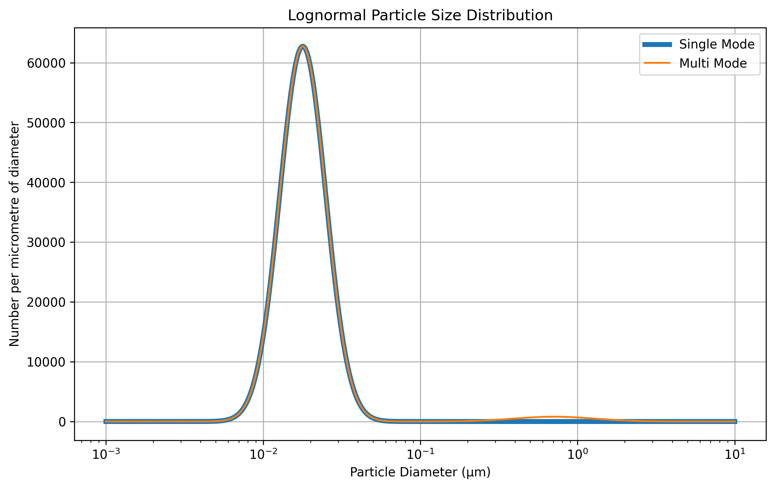
Recover the total with the matching integral
Section titled “Recover the total with the matching integral”The printed integrals use the diameter coordinates, rather than summing the PDF values. Compare them with the supplied totals: 1,000 for the single component and 2,000 for the mixture. This checks the normalization convention; the helper’s explicit normalization means it is not an independent test of physical realism or tail coverage.
Python · section 10
single_mode_total_concentration = np.trapezoid(    single_mode_distribution, x_values)multi_mode_total_concentration = np.trapezoid(multi_mode_distribution, x_values)
print(f"Total Concentration for Single Mode: {single_mode_total_concentration}")print(f"Total Concentration for Multi Mode: {multi_mode_total_concentration}")
Total Concentration for Single Mode: 1000.0
Total Concentration for Multi Mode: 2000.000000000002Convert density to number in each bin
Section titled “Convert density to number in each bin”A bin-integrated distribution stores a contribution
The helper weights the PDF by bin widths and rescales the sum to the requested total. On a logarithmic grid, large-diameter bins are wider in linear diameter, so weighting changes the relative heights. Both plots still describe the same chosen population, within the numerical discretization.
Python · section 11
single_pmf_distribution = par.particles.get_lognormal_pmf_distribution( x_values, single_mode, single_mode_gsd, single_mode_nparticles)multi_pmf_distribution = par.particles.get_lognormal_pmf_distribution( x_values, multi_mode, multi_mode_gsd, multi_mode_nparticles)Read the bin-integrated spectrum
Section titled “Read the bin-integrated spectrum”Compare this plot with the PDF above. Bin width is now included, so peak heights cannot be compared directly across the two ordinates. Refining the grid changes number per bin even when the underlying continuous population is unchanged.
Python · section 12
plt.figure(figsize=(10, 6))plt.plot(x_values, single_pmf_distribution, label="Single Mode", linewidth=4)plt.plot(x_values, multi_pmf_distribution, label="Multi Mode")plt.title("Lognormal PMF Particle Size Distribution")plt.xlabel("Particle Diameter (μm)")plt.ylabel("Number of Particles")plt.xscale("log")plt.legend()plt.grid(True)plt.show()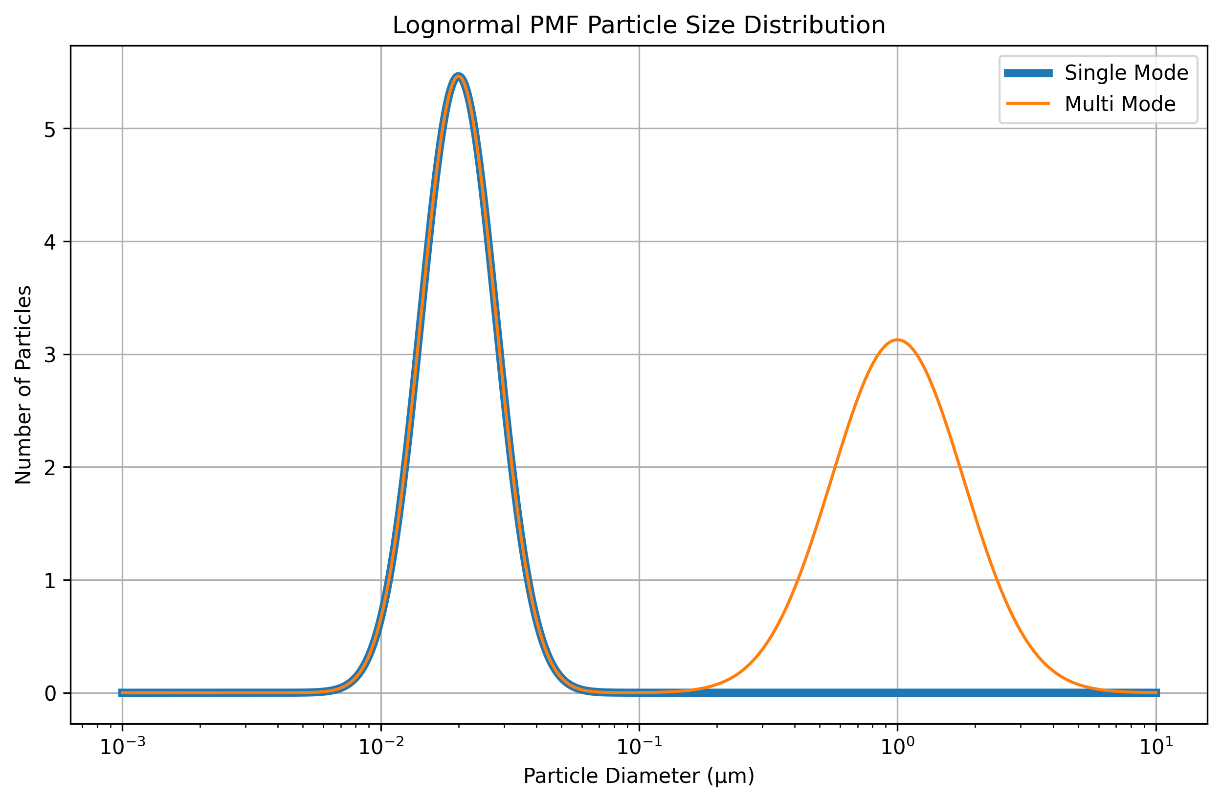
Recover the total with a sum
Section titled “Recover the total with a sum”The PMF is already integrated over bins, so sum its entries without multiplying by bin widths again. The printed values can be compared with the earlier PDF integrals. Agreement checks consistent bookkeeping between representations.
Python · section 14
single_mode_total_concentration = single_pmf_distribution.sum()multi_mode_total_concentration = multi_pmf_distribution.sum()
print(f"Total Concentration for Single Mode: {single_mode_total_concentration}")print(f"Total Concentration for Multi Mode: {multi_mode_total_concentration}")
Total Concentration for Single Mode: 1000.0000000000001
Total Concentration for Multi Mode: 2000.0Carry the measure into the model
Section titled “Carry the measure into the model”The useful distinction is the integration rule: integrate a density against its coordinate, or sum bin contributions. A change in plot shape can therefore come entirely from representation. Before attributing it to aerosol physics, check the coordinate, units, bin widths, and normalization.
Native radius-PDF storage
Section titled “Native radius-PDF storage”Native continuous_pdf storage uses radius
For this final model construction, interpret the supplied component totals as number concentrations in m⁻³. The same numerical spectrum then has units m⁻³ µm⁻¹ before conversion and m⁻⁴ afterward. This concentration convention is an input assumption, not a volume measurement. The radius grid accompanies the stored PDF.
Python · section 15
radius_grid_m = x_values * 1e-6 / 2radius_pdf = multi_mode_distribution * 2e6native_pdf = par.particles.create_particle_data_from_radii( radii=radius_grid_m, concentration=radius_pdf, distribution_type="continuous_pdf", density=1000.0,)print("Native radius-PDF number density [m^-3]:", native_pdf.number_density)Native radius-PDF number density [m^-3]: [2000.]What this lets you compare
Section titled “What this lets you compare”The final printed native number density should retain the mixture’s supplied 2,000 m⁻³ under the stated concentration convention. The key result is that PDF, bin-integrated number, and native radius PDF require different ordinates while preserving the represented population.
To adapt this to an instrument spectrum, first identify whether its ordinate
is
Explore this topic: Size distributions