

Measured CUDA scaling on an RTX 5060
Download Python script · Download script with helper and data files (.zip)
Measured CUDA scaling on an RTX 5060
Section titled “Measured CUDA scaling on an RTX 5060”Would a faster timestep make your whole study faster? Use these measurements to distinguish particle scaling, box scaling, and setup/transfer cost before choosing an execution path. The prepared quick start explains the workflow whose costs are separated here.
This CPU plotting script reads saved, qualified measurements. It does not rerun the GPU campaign. Its small data file contains only plotted point/line summaries and the provenance text shown below, not model states or image arrays. The underlying experiment uses float64, three warmups, seven identical-state timing repetitions, and seven independent fresh runs including setup and download. Brownian legacy timings cover resident work only. Every GPU mode uses actual CUDA.
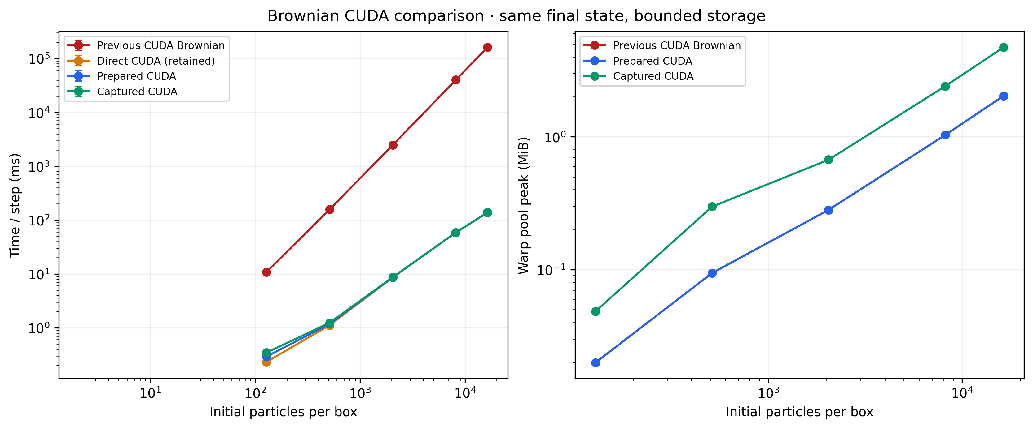
Condensation cases include exponential dilution; the CPU comparison uses the same four fixed condensation substeps and physical configuration. “Direct” means retained low-level kernels without repeated public-wrapper validation. Prepared and captured paths use the public simulation owner. The old/new Brownian comparison is between two GPU implementations, not a CPU speedup. Pair work remains quadratic despite bounded scratch storage.
All ratios below are descriptive measurements of this machine and workload. The minimum–maximum bars show seven-run spread, not confidence intervals. Resident throughput excludes state restoration and analysis; fresh-run time includes preparation, capture when selected, work and download. CUDA context initialization and JIT compilation are warmed before measurement.
Python · section 1
"""Render measured timing and memory without requiring a local GPU."""
import jsonfrom pathlib import Path
import matplotlib.pyplot as pltimport numpy as np
LABELS = {    "numpy": "Native NumPy CPU",    "direct": "Direct CUDA (retained)",    "prepared": "Prepared CUDA",    "captured": "Captured CUDA",    "legacy": "Previous CUDA Brownian",}COLORS = dict(zip(LABELS, ("0.35", "#d97706", "#2563eb", "#059669", "#b91c1c")))

def read_results():    """Load the registry-provided data or the checkout copy."""    paths = (        Path("rtx5060.json"),        Path("docs/data/gpu/rtx5060.json"),    )    path = next((path for path in paths if path.is_file()), None)    if path is None:        raise FileNotFoundError("Download the ZIP containing rtx5060.json")    report = json.loads(path.read_text())    if (        report["schema_version"] != 2        or not report["qualified"]        or report["job_count"] != 104    ):        raise ValueError("The complete 104-job campaign must be qualified")    return report

def curve(ax, rows, mode, x_field, *, timing="resident", throughput=False):    """Plot medians and measured min–max spread with explicit work counts."""    rows = sorted(        (row for row in rows if row["mode"] == mode),        key=lambda row: row["case"][x_field],    )    if not rows:        return    x = [row["case"][x_field] for row in rows]    y, lower, upper = [], [], []    for row in rows:        times = row["timings"][timing]        factor = 1.0        if throughput:            factor = (                row["science"]["initial_active_slots"] * row["case"]["steps"]            )            median = factor / times["median_s"]            low = factor / times["maximum_s"]            high = factor / times["minimum_s"]        else:            median = 1000 * times["median_s"] / row["case"]["steps"]            low = 1000 * times["minimum_s"] / row["case"]["steps"]            high = 1000 * times["maximum_s"] / row["case"]["steps"]        y.append(median)        lower.append(median - low)        upper.append(high - median)    ax.errorbar(        x,        y,        yerr=[lower, upper],        marker="o",        capsize=3,        color=COLORS[mode],        label=LABELS[mode],    )    ax.set(xscale="log", yscale="log")    ax.grid(True, alpha=0.2)
Particle and box scaling
Section titled “Particle and box scaling”The first row holds the box count at one. The second row holds capacity at 1,024 slots per box. Throughput uses initial active particles × timesteps; the small saved series retains only values needed by these graphs. Comparing one huge box with many smaller boxes changes execution geometry, so neither arrangement is a universal predictor for other physics.
Python · section 2
def scaling_figures(rows): """Compare actual execution modes across particle and box counts.""" fig, axes = plt.subplots(2, 2, figsize=(12, 9), constrained_layout=True) for column, family in enumerate(("condensation", "dilution")): selected = [ r for r in rows if r["case"]["name"].startswith(f"particles-{family}-") ] for mode in ("numpy", "direct", "prepared", "captured"): curve(axes[0, column], selected, mode, "slots") axes[0, column].set( title="Condensation + dilution" if column == 0 else "Dilution", xlabel="Active particles in one box", ylabel="Resident time / step (ms)", ) boxes = [r for r in rows if r["case"]["name"].startswith("boxes-")] for mode in ("numpy", "direct", "prepared", "captured"): curve(axes[1, 0], boxes, mode, "boxes") curve(axes[1, 1], boxes, mode, "boxes", throughput=True) axes[1, 0].set(xlabel="Boxes (1,024 slots each)", ylabel="Time / step (ms)") axes[1, 1].set( xlabel="Boxes (1,024 slots each)", ylabel="Initial particle-steps / s" ) axes[0, 0].legend(fontsize=8) fig.suptitle( "RTX 5060 · float64 scaling · median and min–max of seven runs" )Old and new Brownian execution
Section titled “Old and new Brownian execution”Both implementations use the same initial state, persistent random words and selection semantics; all measured modes must produce byte-identical final native aerosol states. Raw RNG continuation is checked separately by the Brownian and checkpoint regression suites. The parallel implementation changes majorant evaluation and retains bounded temporary memory. The curves expose the remaining quadratic cost.
Python · section 3
def brownian_figures(rows): """Separate old/new GPU improvement from native-CPU comparisons.""" selected = [r for r in rows if r["case"]["name"].startswith("brownian-")] fig, axes = plt.subplots(1, 2, figsize=(11, 4.5), constrained_layout=True) for mode in ("legacy", "direct", "prepared", "captured"): curve(axes[0], selected, mode, "slots") axes[0].set(xlabel="Initial particles per box", ylabel="Time / step (ms)") axes[0].legend(fontsize=8) for mode in ("legacy", "prepared", "captured"): group = sorted( (r for r in selected if r["mode"] == mode), key=lambda r: r["case"]["slots"], ) axes[1].loglog( [r["case"]["slots"] for r in group], [r["memory"]["mempool_peak_bytes"] / 2**20 for r in group], "o-", color=COLORS[mode], label=LABELS[mode], ) axes[1].set( xlabel="Initial particles per box", ylabel="Warp pool peak (MiB)" ) axes[1].legend(fontsize=8) axes[1].grid(True, alpha=0.2) fig.suptitle("Brownian CUDA comparison · same final state, bounded storage")Transfer cost, occupancy and physical output
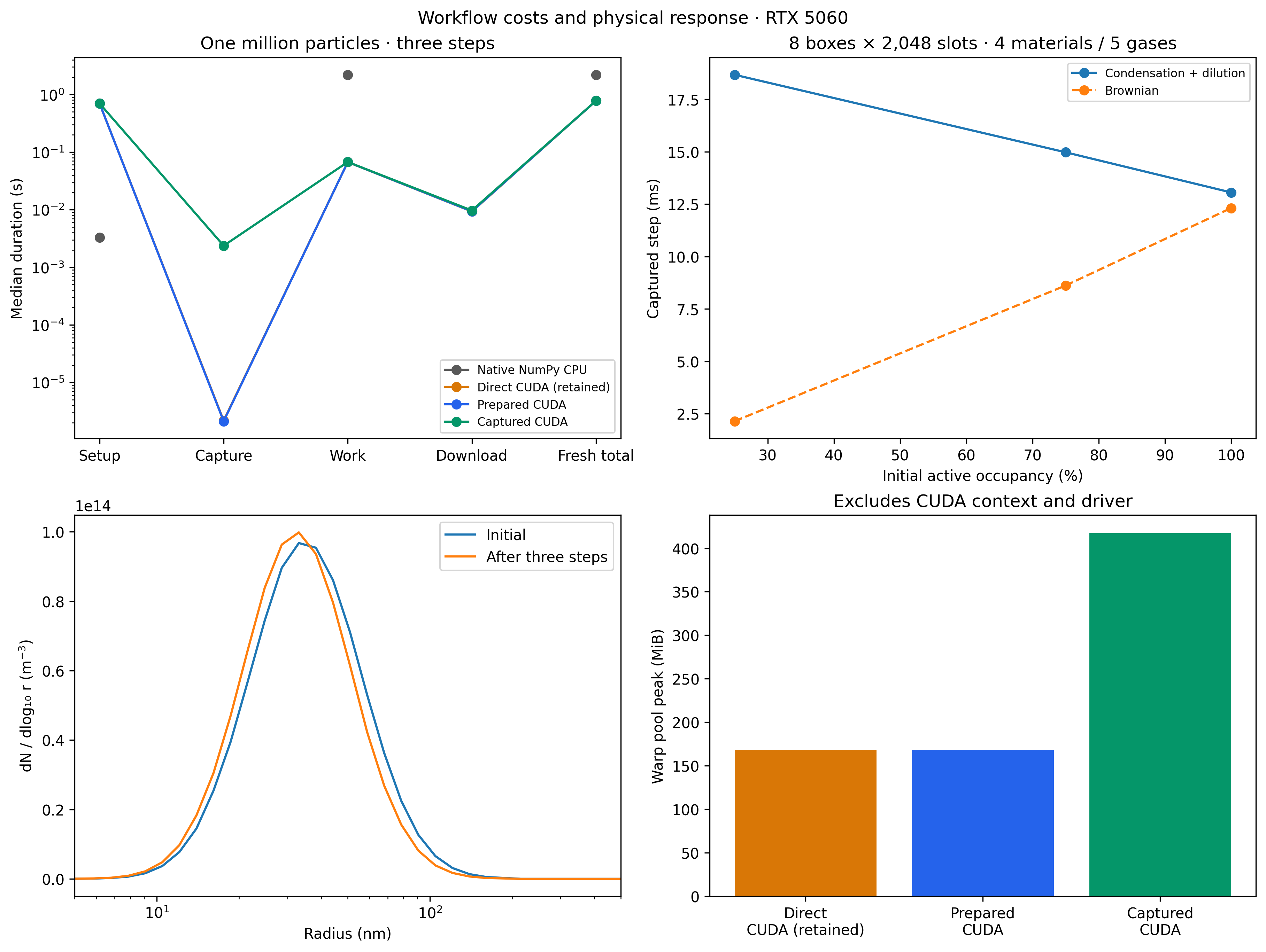
Section titled “Transfer cost, occupancy and physical output”A short million-particle run can spend more time preparing state than advancing it. These costs are reported separately instead of presenting kernel speedup as end-to-end speedup. Component medians come from different timing samples and need not sum to the independently measured total. Zero or inapplicable cost components are omitted from the logarithmic plot. The size distribution is a timing-workload snapshot, not a time-converged prediction. The separate multibox and forcing tutorials test timestep refinement. The occupancy experiment uses four materials, five gases and fixed capacity; fewer active particles do not remove all fixed-capacity work.
Python · section 4
def cost_and_science_figures(rows):    """Show complete-workflow costs alongside variability and a distribution."""    fig, axes = plt.subplots(2, 2, figsize=(12, 9), constrained_layout=True)    selected = [        r for r in rows if r["case"]["name"] == "particles-condensation-1048576"    ]    components = ("setup", "capture", "resident", "download", "end_to_end")    for row in selected:        values = [            row["timings"].get(c, {}).get("median_s", np.nan)            for c in components        ]        values = [value if value > 0 else np.nan for value in values]        axes[0, 0].plot(            range(5),            values,            "o-",            color=COLORS[row["mode"]],            label=LABELS[row["mode"]],        )    axes[0, 0].set(        xticks=range(5),        xticklabels=["Setup", "Capture", "Work", "Download", "Fresh total"],        ylabel="Median duration (s)",        yscale="log",        title="One million particles · three steps",    )    axes[0, 0].legend(fontsize=8)    for family, style in (("condensation", "-"), ("brownian", "--")):        group = sorted(            (                r                for r in rows                if r["mode"] == "captured"                and r["case"]["name"].startswith(f"species-{family}-")            ),            key=lambda r: r["case"]["occupancy"],        )        axes[0, 1].plot(            [100 * r["case"]["occupancy"] for r in group],            [                1000 * r["timings"]["resident"]["median_s"] / r["case"]["steps"]                for r in group            ],            "o" + style,            label="Condensation + dilution"            if family == "condensation"            else "Brownian",        )    axes[0, 1].set(        xlabel="Initial active occupancy (%)",        ylabel="Captured step (ms)",        title="8 boxes × 2,048 slots · 4 materials / 5 gases",    )    axes[0, 1].legend(fontsize=8)    row = next(r for r in selected if r["mode"] == "captured")    edges = np.array(row["radius_edges_m"])    centres = np.sqrt(edges[:-1] * edges[1:]) * 1e9    for key, label in (        ("initial_mean_histogram_number_m3", "Initial"),        ("final_mean_histogram_number_m3", "After three steps"),    ):        axes[1, 0].semilogx(            centres, np.array(row[key]) / np.diff(np.log10(edges)), label=label        )    axes[1, 0].set(        xlabel="Radius (nm)", ylabel="dN / dlog₁₀ r (m$^{-3}$)", xlim=(5, 500)    )    axes[1, 0].legend()    modes = [r for r in selected if r["mode"] != "numpy"]    axes[1, 1].bar(        [LABELS[r["mode"]].replace(" ", "\n", 1) for r in modes],        [r["memory"]["mempool_peak_bytes"] / 2**20 for r in modes],        color=[COLORS[r["mode"]] for r in modes],    )    axes[1, 1].set(        ylabel="Warp pool peak (MiB)", title="Excludes CUDA context and driver"    )    fig.suptitle("Workflow costs and physical response · RTX 5060")

def run_example():    """Render committed measurements and print their exact provenance."""    report = read_results()    rows = report["reports"]    scaling_figures(rows)    brownian_figures(rows)    cost_and_science_figures(rows)    gpu = report["provenance"]    print("GPU:", gpu["gpu_name"], "Warp:", gpu["warp"])    print("CPU:", gpu["cpu_model"])    print("Campaign start:", report["campaign_started_at"])    print("Executable SHA256:", report["executable_sha256"])    print("Source revision:", gpu["source_revision"])    print("Qualified jobs:", report["job_count"])    print("All direct/prepared/captured/legacy CUDA states match exactly.")    print(        "Full-array CPU/CUDA parity cases:",        report["cpu_cuda_parity_case_count"],    )    print("Memory method:", report["memory_method"])    plt.show()    return report

if __name__ == "__main__":    run_example()
Explicit cpu invocation
result = run_example()GPU: NVIDIA GeForce RTX 5060 Warp: 1.11.1
CPU: AMD Ryzen AI 9 HX 370 w/ Radeon 890M
Campaign start: 2026-11-13T23:40:44.667614+00:00
Executable SHA256: c853675d08921a1f7eb2c860ca5650fce0458ec4a31743bc8e64666c29a86ef2
Source revision: 464738b147526193709ba206e51c9b946d375494
Qualified jobs: 104
All direct/prepared/captured/legacy CUDA states match exactly.
Full-array CPU/CUDA parity cases: 17
Memory method: Warp CUDA mempool high-water mark; excludes CUDA context/driver allocations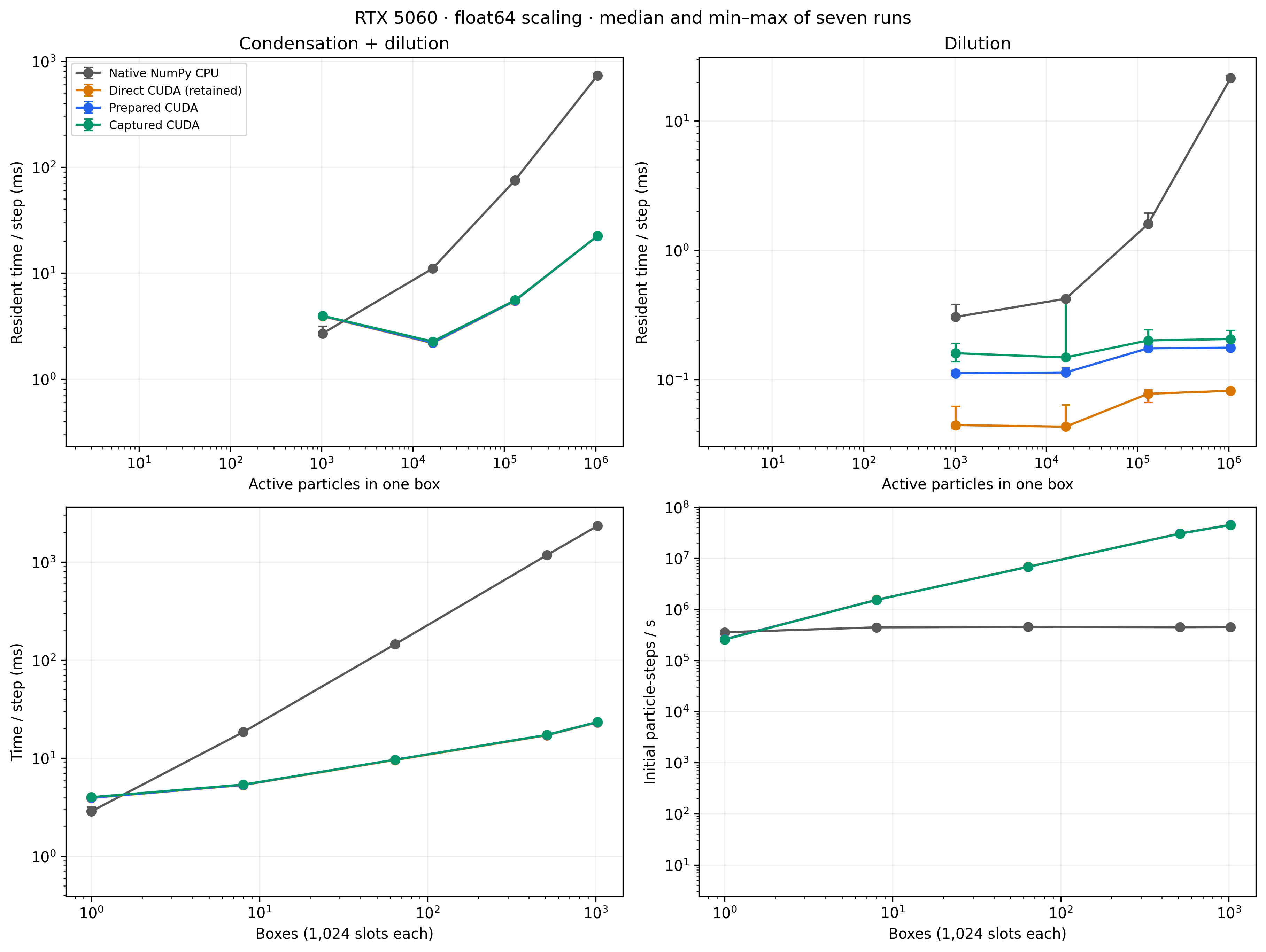
Match the benchmark to the research workload
Section titled “Match the benchmark to the research workload”The plots separate three decisions: how work scales within a box, how many independent boxes can share the device, and whether setup is amortized over enough steps. Smaller retained scratch memory does not remove the quadratic pair work of Brownian coagulation. The plotted distribution is evidence that the timing workload evolved, not a calibrated scientific result.
To budget a parameter sweep, benchmark representative box sizes, occupancies, process schedules, and observation intervals on your device. Report fresh-run time alongside synchronized stepping, retain the same physical checks across backends, and repeat timings. Extrapolating one large-box rate to many small boxes—or this RTX 5060 campaign to another device—needs new measurements.
Explore this topic: Prepared simulations