

Audit a respiratory-droplet illustration before using its predictions
Audit a respiratory-droplet illustration before using its predictions
Section titled “Audit a respiratory-droplet illustration before using its predictions”An evaporation calculation can conserve mass and still represent the wrong materials. This example follows a multicomponent droplet population in initially 30% RH air, while exposing a necessary earlier step: checking that requested chemical names resolve to the intended species.
The retained property lookup fails that identity check. In the saved output, “Lysozyme” resolves to hexachlorophene and “IgA” to isoguanine; the requested calcium and magnesium bicarbonates resolve to carbonates. Those are different substances, not acceptable protein or salt surrogates established by this example. Consequently the results illustrate the workflow and its input-audit failure; they must not be interpreted as quantitative respiratory-droplet or exposure predictions.
Read condensation and evaporation for the mass-transfer mechanism. The useful question here is what additional checks are required before adapting that mechanism to a material mixture.
Python · section 1
# 🚧 Install Particula if you're running this in Google Colab# Remove the comment below to enable installation# Install from the repository root: `python -m pip install -e ".[extra]"`
# 📦 Import necessary librariesimport copy  # to safely duplicate Python objects
import matplotlib.pyplot as plt  # for plottingimport numpy as np  # numerical toolsimport particula as par  # the main Particula packagefrom particula.dynamics.condensation.species_mapping import (    CondensationSpeciesMap,)from particula.execution.gpu_resident_condensation import (    GPUResidentCondensation,)from tqdm import tqdm  # optional: for progress bars during simulation
# 🎨 Set default plot styling using Tailwind-inspired colors from ParticulaTAILWIND = par.util.colors.TAILWINDbase_color = TAILWIND["gray"]["600"]
plt.rcParams.update(    {        "text.color": base_color,        "axes.labelcolor": base_color,        "figure.figsize": (5, 4),        "font.size": 14,        "axes.edgecolor": base_color,        "xtick.color": base_color,        "ytick.color": base_color,        "pdf.fonttype": 42,        "ps.fonttype": 42,    })
Compare requested labels with resolved identities
Section titled “Compare requested labels with resolved identities”The twelve requested labels span water, salts, small organics, and biological materials. The utility first attempts an exact lookup and can fall back to a similar name. Printing the returned name, CAS identifier, and structure is therefore a scientific input check, not merely a status message. The mismatches identified above invalidate the claim that these arrays describe the requested respiratory-fluid composition.
The independently sampled mass ranges are illustrative and lack a cited composition dataset here. Molar masses are kg/mol, densities kg/m³, surface tensions N/m, and vapor pressures Pa. The NaCl surface-tension override is an assumed constant; it is not a concentration-dependent electrolyte model. A verified identity and a numerical property value are separate requirements.
Python · section 2
list_of_chemicals = [    "Water",    "NaCl",    "potassium bicarbonate (KHCO3)",    "potassium dihydrogen phosphate (KH2PO4)",  # K+ + H2PO4–    "calcium bicarbonate [Ca(HCO3)2]",    "magnesium bicarbonate [Mg(HCO3)2]",    "Urea",    "Lactate",    "Glucose",    "Lysozyme",    "IgA",    "cholesterol",]initial_mass_fraction_bounds = [    (0.985, 0.995),  # Water    (0.0006, 0.0023),  # NaCl    (0.0007, 0.0030),  # KHCO3    (0.0002, 0.0027),  # KH2PO4    (0.00002, 0.00045),  # Ca(HCO3)2    (0.000006, 0.00003),  # Mg(HCO3)2    (0.0002, 0.0015),  # Urea    (0.00005, 0.0004),  # Lactate    (0.00001, 0.0002),  # Glucose    (0.000005, 0.00002),  # Lysozyme    (0.00002, 0.0002),  # IgA    (0.00005, 0.0005),  # Cholesterol]
density_array = np.array([])molar_mass_array = np.array([])surface_tension_array = np.array([])short_name = []chemical_dict = {}# Get the CAS numbers for each chemicalfor chem in list_of_chemicals:    cas = par.util.get_chemical_search(chem)    print(f"{chem}: {cas}")    chemical_dict[chem] = par.util.get_chemical_stp_properties(cas)    # Store the molar mass and density    molar_mass_array = np.append(        molar_mass_array, chemical_dict[chem]["molar_mass"]    )    density_array = np.append(density_array, chemical_dict[chem]["density"])    surface_tension_array = np.append(        surface_tension_array, chemical_dict[chem]["surface_tension"]    )    short_name.append(chemical_dict[chem]["name"])
# correct NaCl surface tensionsurface_tension_array[1] = 0.091  # N/m, typical value
# Print the chemical propertiesfor chem, props in chemical_dict.items():    print(f"{chem}:")    print(f"  Name: {props['name']}")    print(f"  CAS: {props['cas_number']}")    print(f"  Smiles: {props['smiles']}")    print(f"  Molar Mass: {props['molar_mass']:.4f} kg/mol")    print(f"  Density: {props['density']:.2f} kg/m³")    print(f"  Surface Tension: {props['surface_tension']} N/m")    print(f"  Vapor Pressure: {props['pure_vapor_pressure']} Pa\n")
Water: WaterNaCl: NaCl
potassium bicarbonate (KHCO3): potassium bicarbonate (KHCO3)
potassium dihydrogen phosphate (KH2PO4): potassium dihydrogen phosphate (KH2PO4)calcium bicarbonate [Ca(HCO3)2]: calcium carbonate [usan]magnesium bicarbonate [Mg(HCO3)2]: magnesium carbonate (mgco3)
Urea: Urea
Lactate: Lactate
Glucose: GlucoseLysozyme: soy-dome
IgA: IgA
cholesterol: cholesterol
Water:
Name: water
CAS: 7732-18-5
Smiles: O
Molar Mass: 0.0180 kg/mol
Density: 997.06 kg/m³
Surface Tension: 0.07197220523022962 N/m
Vapor Pressure: 3169.9293388738784 Pa
NaCl:
Name: sodium chloride
CAS: 7647-14-5
Smiles: [Na+].[Cl-]
Molar Mass: 0.0584 kg/mol
Density: 2169.99 kg/m³
Surface Tension: 0.35290821232462 N/m
Vapor Pressure: 2.245741871175006e-30 Pa
potassium bicarbonate (KHCO3):
Name: potassium bicarbonate
CAS: 298-14-6
Smiles: C(=O)(O)[O-].[K+]
Molar Mass: 0.1001 kg/mol
Density: 2170.00 kg/m³
Surface Tension: None N/m
Vapor Pressure: None Pa
potassium dihydrogen phosphate (KH2PO4):
Name: potassium dihydrogen phosphate
CAS: 7778-77-0
Smiles: OP(=O)(O)[O-].[K+]
Molar Mass: 0.1361 kg/mol
Density: 2340.01 kg/m³
Surface Tension: None N/m
Vapor Pressure: None Pa
calcium bicarbonate [Ca(HCO3)2]:
Name: calcium carbonate
CAS: 471-34-1
Smiles: C(=O)([O-])[O-].[Ca+2]
Molar Mass: 0.1001 kg/mol
Density: 2710.00 kg/m³
Surface Tension: None N/m
Vapor Pressure: None Pa
magnesium bicarbonate [Mg(HCO3)2]:
Name: magnesium carbonate
CAS: 546-93-0
Smiles: C(=O)([O-])[O-].[Mg+2]
Molar Mass: 0.0843 kg/mol
Density: 3010.00 kg/m³
Surface Tension: None N/m
Vapor Pressure: None Pa
Urea:
Name: urea
CAS: 57-13-6
Smiles: C(=O)(N)N
Molar Mass: 0.0601 kg/mol
Density: 932.80 kg/m³
Surface Tension: 0.06630868366869905 N/m
Vapor Pressure: 9.647479358454168 Pa
Lactate:
Name: lactic acid
CAS: 50-21-5
Smiles: CC(C(=O)O)O
Molar Mass: 0.0901 kg/mol
Density: 1146.11 kg/m³
Surface Tension: 0.06892887098077884 N/m
Vapor Pressure: 0.42214021514470007 Pa
Glucose:
Name: glucose
CAS: 50-99-7
Smiles: O=C[C@H](O)[C@@H](O)[C@H](O)[C@H](O)CO
Molar Mass: 0.1802 kg/mol
Density: 1618.57 kg/m³
Surface Tension: 0.10078381855423499 N/m
Vapor Pressure: 3.472643152420593e-11 Pa
Lysozyme:
Name: hexachlorophene
CAS: 70-30-4
Smiles: C1=C(C(=C(C(=C1Cl)Cl)CC2=C(C(=CC(=C2Cl)Cl)Cl)O)O)Cl
Molar Mass: 0.4069 kg/mol
Density: 2009.99 kg/m³
Surface Tension: 0.07787535981784431 N/m
Vapor Pressure: 9.468715811988936e-14 Pa
IgA:
Name: isoguanine
CAS: 3373-53-3
Smiles: C1=NC2=NC(=O)NC(=C2N1)N
Molar Mass: 0.1511 kg/mol
Density: 815.71 kg/m³
Surface Tension: 0.1373263034398279 N/m
Vapor Pressure: 0.00012951501534944908 Pa
cholesterol:
Name: cholesterol
CAS: 57-88-5
Smiles: CC(C)CCC[C@@H](C)[C@H]1CC[C@H]2[C@@H]3CC=C4C[C@@H](O)CC[C@]4(C)[C@H]3CC[C@]12C
Molar Mass: 0.3867 kg/mol
Density: 1064.37 kg/m³
Surface Tension: 0.03942801914463943 N/m
Vapor Pressure: 8.548725890318368e-07 PaDistinguish reproducible inputs from validated inputs
Section titled “Distinguish reproducible inputs from validated inputs”The sample contains 1000 particles at 10⁻⁴ cm⁻³ (100 m⁻³), corresponding to 10 m³ represented volume, at 298.15 K. The fixed sampling seed controls this realization, not the accuracy of the material model.
Missing vapor pressures are replaced by 10⁻³⁰ Pa, making those lanes nearly nonvolatile. Missing surface tensions receive 0.072 N/m. These substitutions allow execution; they do not resolve missing measurements or incorrect identities. Record them as assumptions before interpreting any partitioning.
Python · section 4
# 🎲 Ensure reproducibilitynp.random.seed(100)
# 🔢 Simulation settingsnumber_of_samples = 1_000  # Number of particles to simulatetotal_number_per_cm3 = 1e-4  # Particle number concentration [#/cm³]simulation_volume = (    number_of_samples / total_number_per_cm3 * 1e-6)  # Simulation volume in m³ (converted from cm³)
temperature = 298.15  # System temperature in Kelvin (25°C)
# 🌡 Build vapor pressure strategies for each chemicalvapor_pressure_strategy_list = []
for chem_i, props in chemical_dict.items():    vapor_pressure_temp = props["pure_vapor_pressure"]
    if vapor_pressure_temp is None:        print(f"⚠️ Warning: No vapor pressure data for {chem_i}, using default.")        vapor_pressure_temp = 1e-30  # fallback for non-volatile species
    vapor_pressure_i = (        par.gas.ConstantVaporPressureBuilder()        .set_vapor_pressure(vapor_pressure_temp, "Pa")        .build()    )
    vapor_pressure_strategy_list.append(vapor_pressure_i)
# 💧 Ensure surface tension values are setsurface_tension_array = np.array(    [0.072 if x is None else x for x in surface_tension_array])
⚠️ Warning: No vapor pressure data for potassium bicarbonate (KHCO3), using default.
⚠️ Warning: No vapor pressure data for potassium dihydrogen phosphate (KH2PO4), using default.
⚠️ Warning: No vapor pressure data for calcium bicarbonate [Ca(HCO3)2], using default.
⚠️ Warning: No vapor pressure data for magnesium bicarbonate [Mg(HCO3)2], using default.Initialize a finite gas reservoir at 30% saturation
Section titled “Initialize a finite gas reservoir at 30% saturation”Water gas concentration is 0.3 times its modeled saturation concentration; other vapor lanes start near zero. Gas names retain the requested labels even when property lookup returned another substance, so names in a container do not certify the underlying material identity.
Temperature is fixed at 298.15 K and pressure at 101325 Pa. Humidity is only initialized here. The active loop does not reset it to 30% at each step.
Python · section 5
# 💨 Initialize gas-phase concentrations near zeroconcentration_gas = np.ones(len(list_of_chemicals)) * 1e-30  # kg/m³
# 💧 Set water vapor to 30% RHisat_water = vapor_pressure_strategy_list[0].saturation_concentration(    molar_mass_array[0], temperature)concentration_gas[0] = isat_water * 0.3  # 30% RH
# 🧪 Build gas-phase species with vapor strategies and concentrationsgas_species = par.gas.GasData(    name=list_of_chemicals,    molar_mass=molar_mass_array.copy(),    partitioning=np.ones(len(list_of_chemicals), dtype=bool),    concentration=concentration_gas[None, :].copy(),)environment = par.gas.EnvironmentData(    temperature=np.array([temperature]),    pressure=np.array([101325.0]),    saturation_ratio=np.zeros((1, len(list_of_chemicals))),)
Track what the composition sampling actually constructs
Section titled “Track what the composition sampling actually constructs”The three supplied radius modes are 0.3, 4, and 40 µm with relative weights 15, 2, and 0.2. They define an illustrative sample, not a validated cough-size distribution. Water-equivalent spherical mass is multiplied independently by each sampled composition factor. Those factors are not jointly normalized, so the final total mass and reconstructed radius need not exactly equal the water-only sample from which they were built.
The κ array is assumed, with water in lane zero. Each species receives its own surface-phase label, so this configuration retains species-specific surface tensions rather than averaging them across one shared liquid phase. It does not calculate physical phase separation. The inventory helper counts weighted particle mass plus gas mass in the represented volume.
Python · section 6
# 💠 3a. Lognormal size distributions for cough droplet modes# Modes: bronchiolar, laryngeal, oropharyngealmodes = np.array([0.6, 8.0, 80.0]) / 2 * 1e-6  # radii in metersgeometric_standard_deviations = np.array([1.65, 2.4, 1.6])relative_number = np.array([15, 2, 0.2])  # relative weights
# Generate sampled radiiradii_cough = par.particles.get_lognormal_sample_distribution(    mode=modes,    geometric_standard_deviation=geometric_standard_deviations,    number_of_particles=relative_number,    number_of_samples=number_of_samples,)
# 💧 3b. Assign initial water mass and scale by chemical mass fractionsmass_water = 4 / 3 * np.pi * (radii_cough**3) * density_array[0]
mass_speciation = np.repeat(    mass_water[:, np.newaxis], len(list_of_chemicals), axis=1)
# Apply random mass fractions from defined boundsfor i, (_chem, bounds) in enumerate(    zip(list_of_chemicals, initial_mass_fraction_bounds)):    mass_fraction = np.random.uniform(bounds[0], bounds[1], number_of_samples)    mass_speciation[:, i] *= mass_fraction
# ⚗️ 3c. Define activity strategy using kappa parameterskappa_parameter = np.array(    [0.0, 1.1, 0.6, 0.6, 0.6, 0.6, 0.3, 0.2, 0.1, 0.1, 0.1, 0.01])
activity_strategy = (    par.particles.ActivityKappaParameterBuilder()    .set_molar_mass(molar_mass_array, "kg/mol")    .set_density(density_array, "kg/m^3")    .set_kappa(kappa_parameter)    .set_water_index(0)    .build())
# Define surface tension strategysurface_strategy = (    par.particles.SurfaceStrategyMassBuilder()    .set_surface_tension(surface_tension_array, "N/m")    .set_density(density_array, "kg/m^3")    .set_phase_index(np.arange(len(list_of_chemicals)))    .build())
# 🧱 3d. Build resolved particle objectresolved_masses = par.particles.create_resolved_particle_data(    masses=mass_speciation,    density=density_array,    volume=simulation_volume,)aerosol = par.Aerosol(    particles=resolved_masses, gas=gas_species, environment=environment)

def species_inventory(aero):    """Independent species inventory in kg, including represented volume."""    return np.sum(        aero.particles.masses * aero.particles.concentration[..., None], axis=1    ) + (aero.gas.concentration * aero.particles.volume[:, None])

initial_inventory = species_inventory(aerosol)
# Optional: print summary of aerosol systemprint("Particle slots:", aerosol.particles.masses.shape[1])print("Gas species:", ", ".join(aerosol.gas.name))
Particle slots: 1000
Gas species: Water, NaCl, potassium bicarbonate (KHCO3), potassium dihydrogen phosphate (KH2PO4), calcium bicarbonate [Ca(HCO3)2], magnesium bicarbonate [Mg(HCO3)2], Urea, Lactate, Glucose, Lysozyme, IgA, cholesterolInspect the initialized distribution on its own terms
Section titled “Inspect the initialized distribution on its own terms”The histogram counts sampled radii per logarithmic bin. It is not yet a
number concentration or a diameter spectrum. The native ParticleData stores
the species masses and represented counts; its derived radii include the
sampled composition and densities. This is the appropriate initialized state
to compare with later sizes.
Python · section 7
fig, ax = plt.subplots()
# Log-scale histogram of particle radiiax.hist(    np.log10(aerosol.particles.radii[0]),  # convert to log10    bins=50,    density=False,    alpha=0.5,)
ax.set_xlabel("log₁₀(Radius [m])")ax.set_ylabel("Bin Counts")ax.set_title("Initial Particle Size Distribution")plt.tight_layout()plt.show()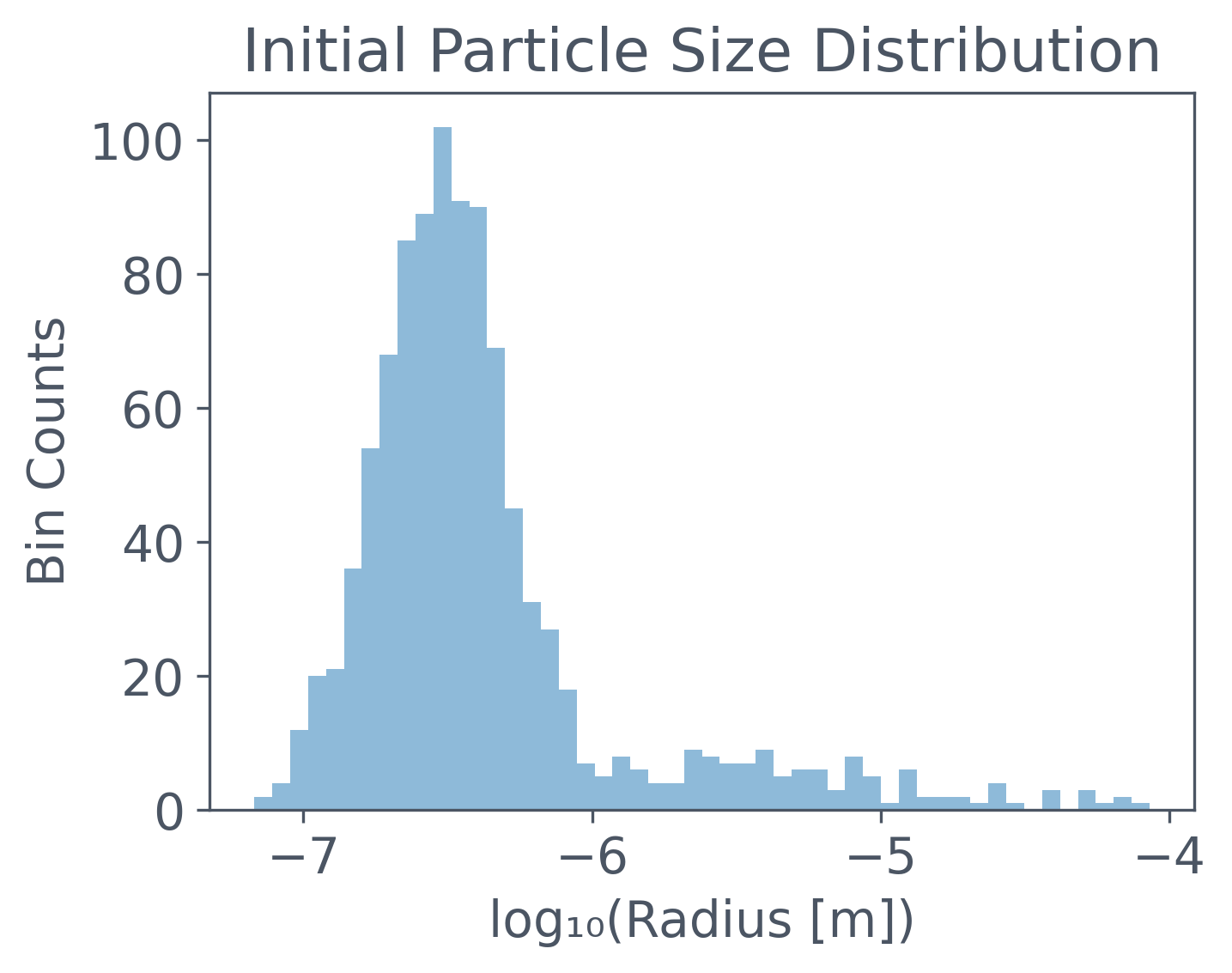
Separate a configured process from an executed process
Section titled “Separate a configured process from an executed process”Condensation/evaporation maps all twelve lanes, with a common diffusivity 2×10⁻⁵ m²/s and accommodation one. These are simplifying assumptions across a chemically diverse set of requested labels. A Brownian process is also constructed, but its execution is commented out in the loop below. The saved calculation therefore contains mass transfer alone, without coagulation, ventilation, sedimentation removal, or temperature feedback.
Python · section 9
# 💧 Isothermal Condensationcondensation_strategy = par.dynamics.CondensationIsothermal(    molar_mass=np.array(molar_mass_array),    activity_strategy=activity_strategy,    surface_strategy=surface_strategy,    vapor_pressure_strategy=vapor_pressure_strategy_list,    species_map=CondensationSpeciesMap(        tuple(gas_species.name),        tuple((i, i) for i in range(len(list_of_chemicals))),    ),    diffusion_coefficient=2e-5,  # typical air value [m²/s]    accommodation_coefficient=1,  # full sticking efficiency    # skip_partitioning_indices=[]      # optional: exclude species)condensation_process = par.dynamics.MassCondensation(condensation_strategy)
# ⚪ Brownian Coagulationcoagulation_strategy = (    par.dynamics.BrownianCoagulationBuilder()    .set_distribution_type("particle_resolved")  # use individual particles    .build())coagulation_process = par.dynamics.Coagulation(coagulation_strategy)
Record 20 seconds of adaptive closed mass transfer
Section titled “Record 20 seconds of adaptive closed mass transfer”There are 201 stored states, including both endpoints of the full 20 s run. ROS3 adapts condensation steps inside each 0.1 s output interval, with rtol 10⁻⁵, particle atol 10⁻²⁵ kg and gas atol 10⁻¹² kg/m³. Water exchanges with a finite gas reservoir. Better integration does not repair uncertain chemical properties or validate respiratory-fluid predictions.
At every stored state, the assertion compares each gas-plus-particle inventory with its initial value at rtol=10⁻¹² and atol=10⁻³⁰ kg. This checks material accounting for the supplied arrays; it cannot detect that a property array belongs to the wrong chemical. Radius-bin counts, bulk particle species masses, and vapor saturation ratios support distinct diagnostics below.
All twelve materials exchange on CUDA. The adaptive clock, acceptance and step-size decisions execute inside a native CUDA conditional graph. Snapshots explicitly download the 201 requested observations. Internal work counts are printed by the run; inventory checks alone do not establish convergence.
Python · section 10
print("Initial gas concentration (kg/m^3):", aerosol.gas.concentration)
# 🔁 Deep copy for simulationaerosol_process = copy.deepcopy(aerosol)
# Simulation parameterstotal_time = 20  # secondstotal_steps = 200
time_step = total_time / total_stepstime_array = np.linspace(0.0, total_time, total_steps + 1)time_len = len(time_array)
# 📊 Initialize arrays for tracking outputsbins_lognormal = np.logspace(-8, -4, 100)distribution_counts = np.zeros((time_len, len(bins_lognormal) - 1))species_mass = np.zeros((time_len, len(list_of_chemicals)))vapor_saturation = np.zeros((time_len, len(list_of_chemicals)))
simulation = GPUResidentCondensation(    aerosol_process,    condensation_strategy,    device="cuda:0",    method="ros3",    rtol=1e-5,    particle_atol=1e-25,    gas_atol=1e-12,    first_step=1e-6,    max_step=time_step,)
# 🌀 Time integration loopfor step, _t in enumerate(    tqdm(time_array, desc="Running Sim", mininterval=0.5)):    if step > 0:        while simulation.time < float(_t):            simulation.step(float(_t))        aerosol_process = simulation.snapshot()
    # Record size distribution    distribution_counts[step, :], edges = np.histogram(        aerosol_process.particles.radii[0].copy(),        bins=bins_lognormal,        density=False,    )
    # Record species mass in particles    species_temp = aerosol_process.particles.masses[0].copy()    species_mass[step, :] = np.sum(        species_temp * aerosol_process.particles.concentration[0, :, None],        axis=0,    )    np.testing.assert_allclose(        species_inventory(aerosol_process),        initial_inventory,        rtol=1e-12,        atol=1e-30,    )
    # Record vapor saturation ratios    vapor_saturation[step, :] = np.array(        [            aerosol_process.gas.concentration[0, i]            / strategy.saturation_concentration(                molar_mass_array[i], aerosol_process.environment.temperature[0]            )            for i, strategy in enumerate(vapor_pressure_strategy_list)        ]    )
# Normalize counts to number concentration (#/m³)concentrations = distribution_counts / simulation_volume
# Final system state and actual adaptive workprint("Final gas concentration (kg/m^3):", aerosol_process.gas.concentration)print("Adaptive condensation work:", simulation.statistics)
Initial gas concentration (kg/m^3): [[6.9110312e-03 1.0000000e-30 1.0000000e-30 1.0000000e-30 1.0000000e-30
1.0000000e-30 1.0000000e-30 1.0000000e-30 1.0000000e-30 1.0000000e-30
1.0000000e-30 1.0000000e-30]]Warp 1.11.1 initialized:
CUDA Toolkit 12.9, Driver 13.4
Devices:
"cpu" : "CPU"
"cuda:0" : "NVIDIA GeForce RTX 5060" (8 GiB, sm_120, mempool enabled)
Kernel cache:
~/.cache/warp/1.11.1Module particula.execution._condensation_ode_kernels 9425cdf load on device 'cuda:0' took 3.52 ms (cached)
Module particula.gpu.kernels.thermodynamics 10b2126 load on device 'cuda:0' took 5.94 ms (cached)
Module particula.gpu.kernels.condensation ad8087d load on device 'cuda:0' took 5.99 ms (cached)
Module particula.execution._adaptive_condensation_physics a3e6636 load on device 'cuda:0' took 5.43 ms (cached)
Module particula.execution._condensation_reservoirs b231d81 load on device 'cuda:0' took 5.95 ms (cached)
Module particula.execution._condensation_device_control 053a506 load on device 'cuda:0' took 3.92 ms (cached)
Module particula.execution._condensation_ros3_kernels d88df3a load on device 'cuda:0' took 5.17 ms (cached)
Module particula.execution._condensation_block_kernels d2447a5 load on device 'cuda:0' took 5.08 ms (cached)Final gas concentration (kg/m^3): [[6.91103209e-03 9.99999850e-31 9.99999848e-31 9.99999847e-31
9.99999848e-31 9.99999849e-31 4.18285543e-13 1.90984831e-14
1.55679389e-24 5.12376933e-28 6.26522875e-18 9.74225658e-20]]
Adaptive condensation work: StepStatistics(accepted=8921, rejected=1, domain_rejected=0, rate_calls=446100, jacobian_calls=8922, time_derivative_calls=0, factorizations=8922, linear_solves=26766)Execution progress
Running Sim:   0%|          | 0/201 [00:00<?, ?it/s]
Running Sim:   1%|          | 2/201 [03:03<5:03:58, 91.65s/it]
Running Sim:   1%|▏         | 3/201 [03:18<3:16:40, 59.60s/it]
Running Sim:   2%|▏         | 4/201 [03:27<2:13:54, 40.79s/it]
Running Sim:   2%|▏         | 5/201 [03:33<1:34:05, 28.81s/it]
Running Sim:   3%|▎         | 6/201 [03:36<1:05:49, 20.25s/it]
Running Sim:   3%|▎         | 7/201 [03:40<48:21, 14.95s/it]
Running Sim:   4%|▍         | 8/201 [03:42<35:28, 11.03s/it]
Running Sim:   4%|▍         | 9/201 [03:44<25:32,  7.98s/it]
Running Sim:   5%|▍         | 10/201 [03:46<20:29,  6.44s/it]
Running Sim:   5%|▌         | 11/201 [03:49<16:42,  5.28s/it]
Running Sim:   6%|▌         | 12/201 [03:52<14:12,  4.51s/it]
Running Sim:   6%|▋         | 13/201 [03:54<12:00,  3.83s/it]
Running Sim:   7%|▋         | 14/201 [03:55<08:52,  2.85s/it]
Running Sim:   7%|▋         | 15/201 [03:56<07:25,  2.39s/it]
Running Sim:   8%|▊         | 16/201 [03:58<06:30,  2.11s/it]
Running Sim:   9%|▉         | 18/201 [03:58<04:01,  1.32s/it]
Running Sim:  10%|▉         | 20/201 [03:59<02:49,  1.07it/s]
Running Sim:  10%|█         | 21/201 [04:00<02:33,  1.17it/s]
Running Sim:  11%|█         | 22/201 [04:01<02:48,  1.06it/s]
Running Sim:  11%|█▏        | 23/201 [04:02<03:12,  1.08s/it]
Running Sim:  12%|█▏        | 25/201 [04:03<02:18,  1.27it/s]
Running Sim:  13%|█▎        | 27/201 [04:04<02:10,  1.34it/s]
Running Sim:  14%|█▍        | 28/201 [04:06<02:31,  1.14it/s]
Running Sim:  14%|█▍        | 29/201 [04:06<02:15,  1.27it/s]
Running Sim:  16%|█▌        | 32/201 [04:07<01:26,  1.96it/s]
Running Sim:  17%|█▋        | 35/201 [04:08<01:04,  2.55it/s]
Running Sim:  18%|█▊        | 37/201 [04:08<01:00,  2.69it/s]
Running Sim:  19%|█▉        | 39/201 [04:10<01:15,  2.13it/s]
Running Sim:  20%|██        | 41/201 [04:11<01:21,  1.96it/s]
Running Sim:  21%|██▏       | 43/201 [04:12<01:25,  1.85it/s]
Running Sim:  22%|██▏       | 45/201 [04:13<01:12,  2.15it/s]
Running Sim:  23%|██▎       | 47/201 [04:13<01:06,  2.32it/s]
Running Sim:  24%|██▍       | 49/201 [04:15<01:13,  2.06it/s]
Running Sim:  25%|██▌       | 51/201 [04:16<01:19,  1.89it/s]
Running Sim:  26%|██▋       | 53/201 [04:17<01:17,  1.92it/s]
Running Sim:  28%|██▊       | 56/201 [04:17<00:56,  2.57it/s]
Running Sim:  30%|██▉       | 60/201 [04:18<00:39,  3.56it/s]
Running Sim:  32%|███▏      | 64/201 [04:19<00:33,  4.08it/s]
Running Sim:  33%|███▎      | 67/201 [04:20<00:44,  2.99it/s]
Running Sim:  34%|███▍      | 69/201 [04:21<00:47,  2.76it/s]
Running Sim:  36%|███▌      | 72/201 [04:22<00:40,  3.17it/s]
Running Sim:  37%|███▋      | 74/201 [04:23<00:41,  3.06it/s]
Running Sim:  38%|███▊      | 76/201 [04:24<00:44,  2.78it/s]
Running Sim:  39%|███▉      | 78/201 [04:24<00:42,  2.90it/s]
Running Sim:  41%|████▏     | 83/201 [04:25<00:27,  4.23it/s]
Running Sim:  44%|████▍     | 88/201 [04:25<00:20,  5.52it/s]
Running Sim:  46%|████▋     | 93/201 [04:26<00:16,  6.59it/s]
Running Sim:  49%|████▉     | 98/201 [04:26<00:13,  7.45it/s]
Running Sim:  51%|█████     | 103/201 [04:27<00:12,  8.10it/s]
Running Sim:  54%|█████▎    | 108/201 [04:27<00:11,  8.44it/s]
Running Sim:  56%|█████▌    | 113/201 [04:28<00:12,  6.84it/s]
Running Sim:  58%|█████▊    | 117/201 [04:30<00:17,  4.90it/s]
Running Sim:  60%|██████    | 121/201 [04:31<00:15,  5.12it/s]
Running Sim:  64%|██████▎   | 128/201 [04:31<00:10,  6.85it/s]
Running Sim:  67%|██████▋   | 135/201 [04:32<00:07,  8.36it/s]
Running Sim:  71%|███████   | 142/201 [04:32<00:06,  9.62it/s]
Running Sim:  74%|███████▍  | 149/201 [04:33<00:04, 10.63it/s]
Running Sim:  78%|███████▊  | 156/201 [04:33<00:03, 11.41it/s]
Running Sim:  81%|████████  | 163/201 [04:34<00:03, 11.99it/s]
Running Sim:  85%|████████▍ | 170/201 [04:34<00:02, 12.42it/s]
Running Sim:  88%|████████▊ | 177/201 [04:35<00:01, 12.73it/s]
Running Sim:  92%|█████████▏| 184/201 [04:35<00:01, 12.96it/s]
Running Sim:  95%|█████████▌| 191/201 [04:36<00:00, 13.12it/s]
Running Sim:  99%|█████████▊| 198/201 [04:36<00:00, 13.24it/s]
Running Sim: 100%|██████████| 201/201 [04:36<00:00,  1.38s/it]
Compare initial and final sizes
Section titled “Compare initial and final sizes”The dashed and solid curves use the same radius bins. Their vertical values are number concentration per bin in m⁻³, not dN/dr. A shift toward smaller radii is consistent with net evaporation under the modeled inputs; it does not by itself prove equilibrium or a validated droplet lifetime. Particles moving outside the histogram’s limits would also change the plotted bin sum.
Python · section 11
fig, ax = plt.subplots(figsize=(7, 5))
# Get radii before and after simulationinitial_distribution = aerosol.particles.radii[0].copy()final_distribution = aerosol_process.particles.radii[0].copy()
# Compute binned countscounts_initial, _ = np.histogram(    initial_distribution, bins=bins_lognormal, density=False)counts_final, _ = np.histogram(    final_distribution, bins=bins_lognormal, density=False)
# Plot initial distributionax.plot(    bins_lognormal[:-1],    counts_initial / simulation_volume,    label="Initial Size Distribution",    color=TAILWIND["sky"]["800"],    linestyle="--",)
# Plot final distributionax.plot(    bins_lognormal[:-1],    counts_final / simulation_volume,    label="Final Size Distribution",    color=TAILWIND["rose"]["400"],    linestyle="-",)
# Set axis scales and labelsax.set_xscale("log")ax.set_xlabel("Particle Radius (m)")ax.set_ylabel("Concentration (#/m⁻³)")ax.legend()plt.tight_layout()plt.show()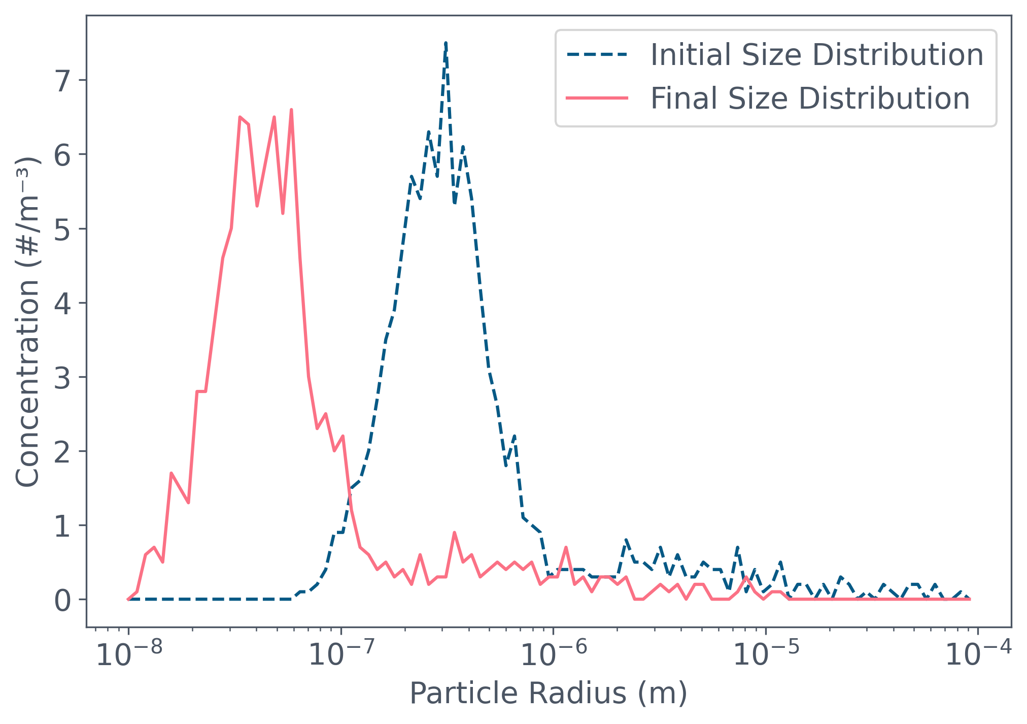
Read gas saturation separately from particle equilibrium
Section titled “Read gas saturation separately from particle equilibrium”The water saturation ratio divides gas concentration by pure-water saturation concentration at the fixed temperature. Unity means saturation relative to that reference, not equilibrium for every curved, multicomponent particle.
The small reservoir change in the saved run reflects this population’s low loading relative to gas water. It is an outcome of the chosen volume and concentrations, not a general claim that humidity stays constant near a cough. The lower axis limit is 0.3, so inspect the actual vertical scale when judging the change.
Python · section 12
fig, ax = plt.subplots(figsize=(7, 5))
# Plot water vapor saturation ratio (species index 0)ax.plot(    time_array,    vapor_saturation[:, 0],    color=TAILWIND["sky"]["800"],    label="Vapor Saturation Ratio (Water)",)
ax.set_ylim(bottom=0.3)ax.set_xlabel("Time (s)")ax.set_ylabel("Vapor Saturation Ratio")ax.set_title("Vapor Saturation Ratio for Water Over Time")ax.legend()
plt.tight_layout()plt.show()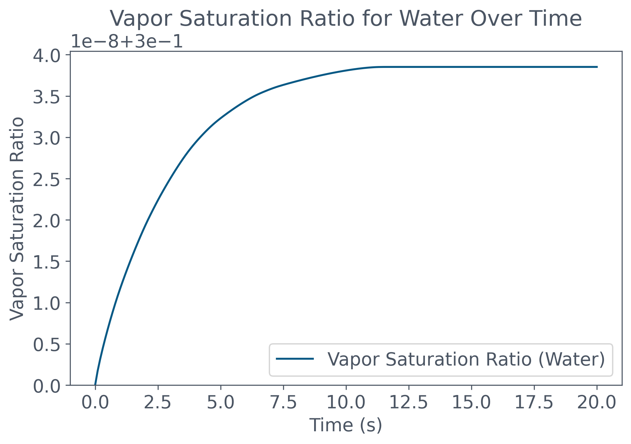
Identify the weighting behind a composition plot
Section titled “Identify the weighting behind a composition plot”The stack plot divides summed particle species mass by summed total particle mass. It is a bulk mass fraction, not an arithmetic average of each particle’s composition, despite the retained “Mean” axis label. Larger particles can dominate this diagnostic. It cannot on its own identify which size class retains water longer.
Legend names come from the resolved property entries. Their disagreement with the requested labels is further evidence of the identity problem, not a change of species caused by evaporation.
Python · section 13
# Compute total mass fraction over timemass_fraction = species_mass / np.sum(species_mass, axis=1, keepdims=True)
# Set color palette (one color per species)color_list = [    TAILWIND["sky"]["800"],  # Water    TAILWIND["rose"]["400"],  # NaCl    TAILWIND["red"]["800"],  # KHCO3    TAILWIND["red"]["600"],  # KH2PO4    TAILWIND["amber"]["500"],  # Ca(HCO3)2    TAILWIND["orange"]["400"],  # Mg(HCO3)2    TAILWIND["teal"]["900"],  # Urea    TAILWIND["teal"]["700"],  # Lactate    TAILWIND["green"]["500"],  # Glucose    TAILWIND["indigo"]["600"],  # Lysozyme    TAILWIND["indigo"]["400"],  # IgA    TAILWIND["cyan"]["500"],  # Cholesterol]
# Create stackplot of species mass fractionfig, ax = plt.subplots(figsize=(8, 5))ax.stackplot(    time_array,    mass_fraction.T,  # Each row = one species    labels=short_name,  # Species names    colors=color_list,    alpha=1.0,)
ax.set_xlabel("Time (s)")ax.set_ylabel("Mean Mass Fraction in Particles")ax.set_ylim(0, 1)ax.grid(True)ax.legend(    title="Species",    loc="lower left",    framealpha=0.9,    fontsize=10,)plt.tight_layout()plt.show()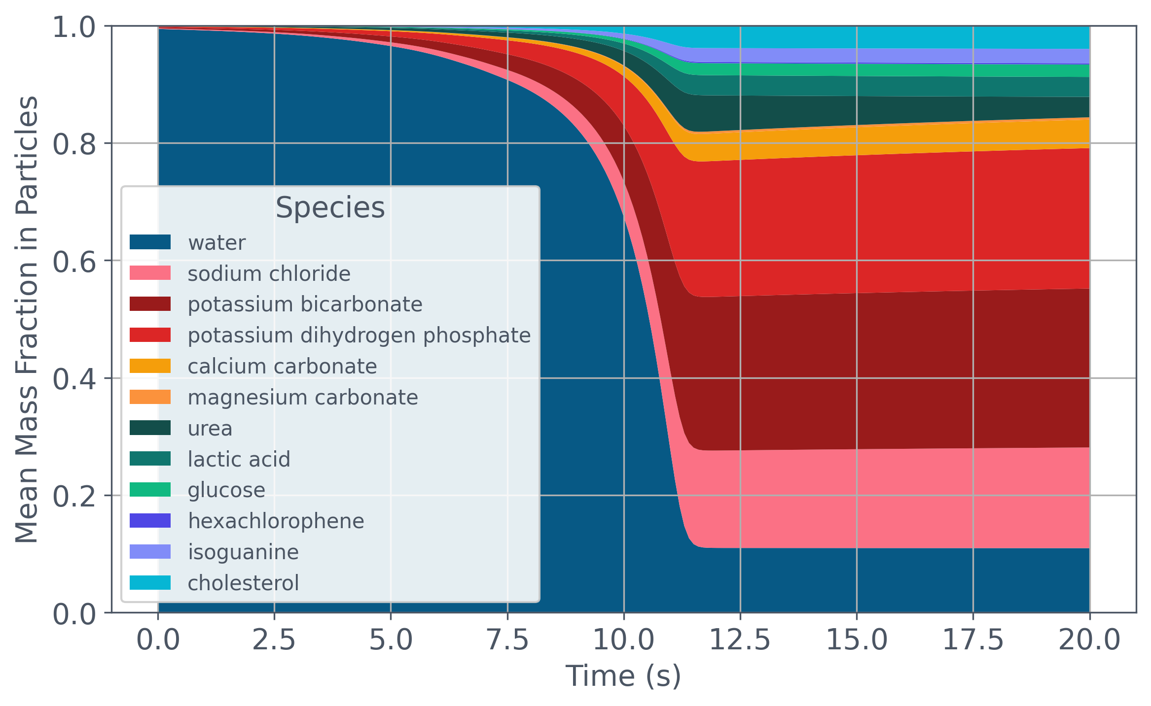
Follow size redistribution without overinterpreting a plateau
Section titled “Follow size redistribution without overinterpreting a plateau”The contour displays log₁₀ of number concentration per radius bin through time. It complements the bulk mass-fraction plot by retaining size information. A slowly changing band is not sufficient evidence of thermodynamic equilibrium; that would require examining mass-transfer rates and convergence as well. The plotted range omits radii below 0.1 µm even though the stored histogram extends lower.
Python · section 14
fig, ax = plt.subplots(figsize=(7, 5))
# Create 2D mesh grid for time and particle radiusX, Y = np.meshgrid(time_array, edges[:-1])
# Convert number concentration to log10 scale (avoid log(0) issues)log_conc = np.log10(    concentrations,    where=concentrations > 0,    out=np.full_like(concentrations, np.nan),  # mask zeros)
# Contour plot of log concentrationcont = ax.contourf(X, Y, log_conc.T)
# Axis settingsax.set_yscale("log")ax.set_ylim(1e-7, 1e-4)ax.set_xlabel("Time (s)")ax.set_ylabel("Particle Radius (m)")
# Add colorbarfig.colorbar(cont, label="Log₁₀ Number Concentration")plt.tight_layout()plt.show()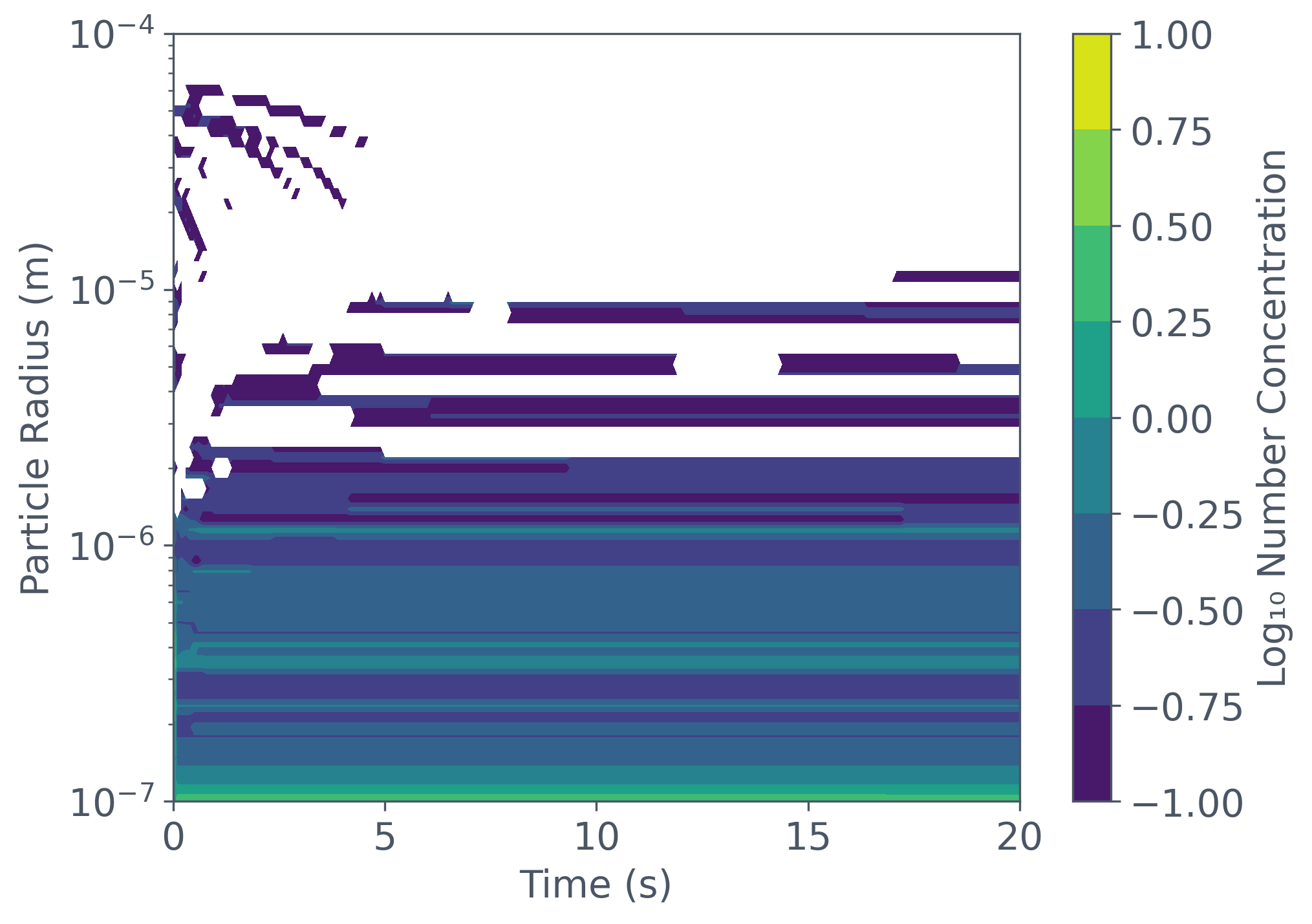
Carry forward the audit, not an unsupported material prediction
Section titled “Carry forward the audit, not an unsupported material prediction”The workflow links sampled composition, finite-reservoir evaporation, and size and mass diagnostics. Its inventory checks pass for the supplied numerical species, but the identity mismatches prevent interpreting those results as respiratory-fluid behavior. Successful execution is not material validation.
Before a research adaptation, replace fuzzy matches with verified identifiers and documented properties or explicitly justified macromolecular surrogates. Normalize the intended starting composition, choose a defensible activity and surface model, then rerun the full calculation. Compare size-resolved water loss across humidity and timestep, using measured evaporation data to test the material assumptions. None of that validation is supplied by the retained run.
Explore this topic: Emissions and exposure