

Separate water cycling from seed loss in a chamber
Separate water cycling from seed loss in a chamber
Section titled “Separate water cycling from seed loss in a chamber”After repeated wet–dry forcing, how much of a droplet’s change comes from water exchange and how much from removal of its dry seed? Extend the single-cycle example to four cycles and three compositions: ammonium sulfate, sucrose, and particles containing both.
Every cycle has 30 s of humid evolution and 60 s of dry evolution at dt=0.1 s, for 360 s in total. Vapor is reset at phase boundaries, not held at constant RH. Condensation and wall removal are active; dilution and coagulation are absent. The comparison is a fixed-step illustration with sampled populations, not a converged activation-threshold study or a calibrated chamber experiment.
Define the chamber and the reservoir resets
Section titled “Define the chamber and the reservoir resets”A 1 m × 0.5 m × 0.5 m geometry matches the 0.25 m³ represented volume. Temperature remains 298.15 K and pressure 101325 Pa. The vapor reset targets are 100.4% saturation for humid phases and 75% for dry phases; water can then move between gas and particles. The wall eddy parameter is 0.001 s⁻¹. A sampling seed and an explicit wall-loss generator make the configured realization repeatable, not statistically representative by themselves.
Python · section 1
import copy
import matplotlib.pyplot as pltimport numpy as npimport particula as parfrom particula.dynamics.condensation.species_mapping import (    CondensationSpeciesMap,)from particula.execution.splitting import condensation_flow
# Optional: uncomment if many steps and you want a progress bar# from tqdm import tqdm
# Plot style (Tailwind gray palette)TAILWIND = par.util.colors.TAILWINDbase_color = TAILWIND["gray"]["600"]plt.rcParams.update(    {        "text.color": base_color,        "axes.labelcolor": base_color,        "figure.figsize": (5, 4),        "font.size": 14,        "axes.edgecolor": base_color,        "xtick.color": base_color,        "ytick.color": base_color,        "pdf.fonttype": 42,        "ps.fonttype": 42,        "savefig.dpi": 150,    })
np.random.seed(100)  # reproducibility for sampling and wall-loss RNG
Keep the integration clock and inventory boundaries aligned
Section titled “Keep the integration clock and inventory boundaries aligned”run_cycle() derives update counts from duration/dt and records physical times
at that same interval. run_multi_cycle() carries the final state into the next
cycle, resetting only the prescribed gas water at each phase boundary. It removes
duplicate boundary records while retaining the full elapsed duration.
Before and after every condensation update, compare mapped gas-plus-particle mass at rtol=10⁻¹² and atol=10⁻³⁰ kg. Wall removal follows that closed update; humidity resets are external water exchanges. A count-dilution helper is tested separately but never applied. Changing its unused coefficient does not alter these histories.
Python · section 2
# Common setup for all scenariostemperature = 298.15  # Ktotal_pressure = 101325.0  # Pachamber_volume = 0.25  # m^3chamber_dims = (1.0, 0.5, 0.5)  # meters
# Calculate water vapor concentrations for RH targetsp_sat_water = par.gas.get_buck_vapor_pressure(temperature)  # PaR_gas = 8.314  # J/(mol*K)molar_mass_water = 0.018015  # kg/molc_sat_water = p_sat_water * molar_mass_water / (R_gas * temperature)  # kg/m^3
# RH targets and corresponding water concentrationsrh_humid_target = 1.004  # 100.4% RH - supersaturatedrh_dry_target = 0.75  # 75% RH - subsaturatedc_water_humid = rh_humid_target * c_sat_waterc_water_dry = rh_dry_target * c_sat_water
print(f"Saturation vapor pressure: {p_sat_water:.1f} Pa")print(f"Saturation concentration: {c_sat_water * 1e3:.4f} g/m^3")print(    f"Humid phase concentration (RH={rh_humid_target}): {c_water_humid * 1e3:.4f} g/m^3")print(    f"Dry phase concentration (RH={rh_dry_target}): {c_water_dry * 1e3:.4f} g/m^3")
# Rectangular wall-loss strategy (shared by all scenarios)wall_loss_strategy = (    par.dynamics.RectangularWallLossBuilder()    .set_chamber_dimensions(chamber_dims)    .set_wall_eddy_diffusivity(0.001, "1/s")    .set_distribution_type("particle_resolved")    .build())wall_loss = par.dynamics.WallLoss(wall_loss_strategy=wall_loss_strategy)
Saturation vapor pressure: 3168.5 Pa
Saturation concentration: 23.0275 g/m^3
Humid phase concentration (RH=1.004): 23.1196 g/m^3
Dry phase concentration (RH=0.75): 17.2707 g/m^3Python · section 3
def apply_count_dilution(    particle_counts: np.ndarray,    dilution_coefficient: float,    dt: float,) -> np.ndarray:    """Illustrate exponential dilution of represented counts, not size.
    This arithmetic reference is not applied to the cycle histories below.    The published cycles contain condensation and wall loss only. For a    complete all-gas/particle dilution runnable see cpu_dilution.py.    """    dilution_factor = np.exp(-dilution_coefficient * dt)    return particle_counts * dilution_factor

def run_cycle(    aerosol: par.Aerosol,    condensation: par.dynamics.MassCondensation,    wall_loss: par.dynamics.WallLoss,    humid_duration: int = 30,    dry_duration: int = 60,    dilution_coefficient: float = 0.01,    c_water_humid: float = 0.023,    c_water_dry: float = 0.015,    water_index: int = 2,    time_offset: float = 0.0,    dt: float = 1.0,) -> tuple:    """Run one activation-deactivation cycle.
    Args:        aerosol: Current aerosol state.        condensation: MassCondensation runnable.        wall_loss: WallLoss runnable.        humid_duration: Duration of humid phase in seconds.        dry_duration: Duration of dry phase in seconds.        dilution_coefficient: Unused reference coefficient; dilution is disabled in this scenario.        c_water_humid: Water vapor concentration during humid phase (kg/m^3).        c_water_dry: Water vapor concentration during dry phase (kg/m^3).        water_index: Index of water species in partitioning_species array.        time_offset: Starting time for this cycle (seconds).        dt: Time step in seconds.
    Returns:        Tuple of (final_aerosol, history_list).    """    if not np.isfinite(dt) or dt <= 0:        raise ValueError("dt must be finite and positive")    humid_steps = round(humid_duration / dt)    dry_steps = round(dry_duration / dt)    np.testing.assert_allclose(        [humid_steps * dt, dry_steps * dt],        [humid_duration, dry_duration],        rtol=0,        atol=1e-12,        err_msg="Phase durations must be whole multiples of dt",    )    history = []    growth = condensation_flow(        "water_exchange",        condensation.condensation_strategy,        method="ros3",        rtol=1e-5,        particle_atol=1e-25,        gas_atol=1e-12,        first_step=1e-6,        max_step=dt,    )
    # Set initial humid phase water concentration    aerosol.gas.concentration[0, water_index] = c_water_humid
    # Record initial state    history.append(        {            "time": 0.0,            "phase": "humid",            "masses": aerosol.particles.masses[0].copy(),        }    )
    # Phase 1: Humid (activation)    for t_step in range(1, humid_steps + 1):        # Condensation handles mass transfer and updates gas concentration internally        before = np.sum(            aerosol.particles.masses            * aerosol.particles.concentration[..., None],            axis=1,        ) + (            aerosol.gas.concentration[:, :-1]            * aerosol.particles.volume[:, None]        )        accepted = growth.advance(aerosol, time_offset + (t_step - 1) * dt, dt)        aerosol.particles.masses[:] = accepted.particles.masses        aerosol.gas.concentration[:] = accepted.gas.concentration        after = np.sum(            aerosol.particles.masses            * aerosol.particles.concentration[..., None],            axis=1,        ) + (            aerosol.gas.concentration[:, :-1]            * aerosol.particles.volume[:, None]        )        np.testing.assert_allclose(after, before, rtol=1e-12, atol=1e-30)        aerosol = wall_loss.execute(aerosol, time_step=dt)        history.append(            {                "time": t_step * dt,                "phase": "humid",                "masses": aerosol.particles.masses[0].copy(),            }        )
    # Phase 2: Dry (deactivation + wall loss)    # Set dry phase water concentration at phase transition    aerosol.gas.concentration[0, water_index] = c_water_dry
    for t_step in range(1, dry_steps + 1):        # Retain the published condensation + wall-loss scenario. Dilution        # is disabled; the separate count-decay exercise is not applied here.        before = np.sum(            aerosol.particles.masses            * aerosol.particles.concentration[..., None],            axis=1,        ) + (            aerosol.gas.concentration[:, :-1]            * aerosol.particles.volume[:, None]        )        accepted = growth.advance(            aerosol, time_offset + humid_duration + (t_step - 1) * dt, dt        )        aerosol.particles.masses[:] = accepted.particles.masses        aerosol.gas.concentration[:] = accepted.gas.concentration        after = np.sum(            aerosol.particles.masses            * aerosol.particles.concentration[..., None],            axis=1,        ) + (            aerosol.gas.concentration[:, :-1]            * aerosol.particles.volume[:, None]        )        np.testing.assert_allclose(after, before, rtol=1e-12, atol=1e-30)        aerosol = wall_loss.execute(aerosol, time_step=dt)        history.append(            {                "time": humid_duration + t_step * dt,                "phase": "dry",                "masses": aerosol.particles.masses[0].copy(),            }        )
    assert len(history) == humid_steps + dry_steps + 1    # Check the elapsed clock before adding a large absolute offset: adjacent    # absolute timestamps can lose precision when subtracted in later cycles.    np.testing.assert_allclose(        np.diff([record["time"] for record in history]), dt, rtol=0, atol=1e-12    )    for record in history:        record["time"] += time_offset    return aerosol, history

def run_multi_cycle(    aerosol: par.Aerosol,    condensation: par.dynamics.MassCondensation,    wall_loss: par.dynamics.WallLoss,    n_cycles: int = 4,    humid_duration: int = 30,    dry_duration: int = 60,    dilution_coefficient: float = 0.01,    c_water_humid: float = 0.023,    c_water_dry: float = 0.015,    water_index: int = 2,    dt: float = 1.0,) -> tuple:    """Run N activation-deactivation cycles sequentially.
    Args:        aerosol: Initial aerosol state (will be deep-copied).        condensation: MassCondensation runnable.        wall_loss: WallLoss runnable.        n_cycles: Number of cycles to run.        humid_duration: Duration of humid phase per cycle (seconds).        dry_duration: Duration of dry phase per cycle (seconds).        dilution_coefficient: Unused reference coefficient; dilution is disabled in this scenario.        c_water_humid: Water vapor concentration during humid phase (kg/m^3).        c_water_dry: Water vapor concentration during dry phase (kg/m^3).        water_index: Index of water species.        dt: Time step in seconds.
    Returns:        Tuple of (final_aerosol, full_history).    """    # Deep copy to avoid mutating original    aerosol_state = copy.deepcopy(aerosol)    full_history = []    cycle_duration = humid_duration + dry_duration
    for cycle in range(n_cycles):        time_offset = cycle * cycle_duration        aerosol_state, cycle_history = run_cycle(            aerosol=aerosol_state,            condensation=condensation,            wall_loss=wall_loss,            humid_duration=humid_duration,            dry_duration=dry_duration,            dilution_coefficient=dilution_coefficient,            c_water_humid=c_water_humid,            c_water_dry=c_water_dry,            water_index=water_index,            time_offset=time_offset,            dt=dt,        )        # Append history (skip first record after first cycle to avoid duplicates)        if cycle == 0:            full_history.extend(cycle_history)        else:            full_history.extend(cycle_history[1:])
    return aerosol_state, full_history

print("Multi-cycle framework functions defined.")
Multi-cycle framework functions defined.Scenario A: one hygroscopic seed material
Section titled “Scenario A: one hygroscopic seed material”Use 1000 ammonium-sulfate seeds sampled around a 100 nm mode radius with geometric standard deviation 1.5. Their κ is 0.61; water occupies lane 1 and starts at zero particle mass. The constant water-like surface tension and fixed material properties are assumptions. The shared constructor adds air as an unmapped gas lane and maps the condensing particle species explicitly.
Python · section 4
def build_native_scenario(    names, masses, density, molar_mass, activity, surface):    """Configure native ordered gas, environment, particles and condensation."""    width = len(names)    gas = par.gas.GasData(        name=[*names, "air"],        molar_mass=np.append(molar_mass, 0.029),        partitioning=np.array([True] * width + [False]),        concentration=np.array(            [[*([1e-30] * (width - 1)), c_water_humid, 1.2]]        ),    )    environment = par.gas.EnvironmentData(        temperature=np.array([temperature]),        pressure=np.array([total_pressure]),        saturation_ratio=np.zeros((1, width + 1)),    )    particles = par.particles.create_resolved_particle_data(        masses=masses,        density=density,        volume=chamber_volume,    )    vapor = [par.gas.ConstantVaporPressureStrategy(1e-30) for _ in names[:-1]]    vapor += [        par.gas.WaterBuckVaporPressureBuilder().build(),        par.gas.ConstantVaporPressureStrategy(101325.0),    ]    strategy = par.dynamics.CondensationIsothermalStaggered(        molar_mass=gas.molar_mass.copy(),        diffusion_coefficient=2.4e-5,        accommodation_coefficient=1.0,        theta_mode="random",        random_state=42,        update_gases=True,        activity_strategy=activity,        surface_strategy=surface,        vapor_pressure_strategy=vapor,        species_map=CondensationSpeciesMap(            tuple(gas.name), tuple((i, i) for i in range(width))        ),    )    return par.Aerosol(        particles=particles, gas=gas, environment=environment    ), strategy

np.random.seed(42)wall_loss_strategy.random_generator = np.random.default_rng(42)
# Scenario A: Ammonium Sulfate only (2 species: AS, water)kappa_as = np.array([0.61, 0.0])density_as = np.array([1770.0, 997.0])molar_mass_as = np.array([0.13214, 0.018015])
activity_strategy_as = (    par.particles.ActivityKappaParameterBuilder()    .set_kappa(kappa_as)    .set_density(density_as, "kg/m^3")    .set_molar_mass(molar_mass_as, "kg/mol")    .set_water_index(1)    .build())
surface_strategy_as = (    par.particles.SurfaceStrategyVolumeBuilder()    .set_surface_tension(0.072, "N/m")    .set_density(density_as, "kg/m^3")    .build())
# Sample particle radii from lognormal distributionn_particles_as = 1000dry_radius_as = par.particles.get_lognormal_sample_distribution(    mode=np.array([100e-9]),  # 100 nm mode radius    geometric_standard_deviation=np.array([1.5]),    number_of_particles=np.array([1.0]),    number_of_samples=n_particles_as,)
# Seed masses from sampled radiivolume_per_particle_as = 4 / 3 * np.pi * dry_radius_as**3ammonium_sulfate_mass_as = volume_per_particle_as * density_as[0]  # 100% ASwater_mass_as = np.zeros_like(dry_radius_as)seed_mass_as = np.stack([ammonium_sulfate_mass_as, water_mass_as], axis=1)
# Create 2-species gas (AS and water) to match particle speciesaerosol_as, condensation_strategy_as = build_native_scenario(    ["ammonium_sulfate", "water"],    seed_mass_as,    density_as,    molar_mass_as,    activity_strategy_as,    surface_strategy_as,)condensation_as = par.dynamics.MassCondensation(    condensation_strategy=condensation_strategy_as)
print("Scenario A (AS-only) configured")print(    f"{aerosol_as.particles.masses.shape[1]} slots; gases: {aerosol_as.gas.name}")
Scenario A (AS-only) configured
1000 slots; gases: ['ammonium_sulfate', 'water', 'air']Scenario B: change the material, and note the sampling difference
Section titled “Scenario B: change the material, and note the sampling difference”Sucrose uses κ=0.10 and its own density and molar mass, with the same nominal size-distribution parameters. It receives a separate radius sample rather than identical radii paired with Scenario A. Differences therefore combine composition and sampling. A controlled κ-only experiment would retain the same initial sizes and other properties.
Python · section 5
# Scenario B: Sucrose only (2 species: sucrose, water)kappa_sucrose = np.array([0.10, 0.0])density_sucrose = np.array([1587.0, 997.0])molar_mass_sucrose = np.array([0.3423, 0.018015])
activity_strategy_sucrose = (    par.particles.ActivityKappaParameterBuilder()    .set_kappa(kappa_sucrose)    .set_density(density_sucrose, "kg/m^3")    .set_molar_mass(molar_mass_sucrose, "kg/mol")    .set_water_index(1)    .build())
surface_strategy_sucrose = (    par.particles.SurfaceStrategyVolumeBuilder()    .set_surface_tension(0.072, "N/m")    .set_density(density_sucrose, "kg/m^3")    .build())
# Sample particle radii from lognormal distributionn_particles_sucrose = 1000dry_radius_sucrose = par.particles.get_lognormal_sample_distribution(    mode=np.array([100e-9]),  # 100 nm mode radius    geometric_standard_deviation=np.array([1.5]),    number_of_particles=np.array([1.0]),    number_of_samples=n_particles_sucrose,)
# Seed masses from sampled radiivolume_per_particle_sucrose = 4 / 3 * np.pi * dry_radius_sucrose**3sucrose_mass_sucrose = (    volume_per_particle_sucrose * density_sucrose[0])  # 100% sucrosewater_mass_sucrose = np.zeros_like(dry_radius_sucrose)seed_mass_sucrose = np.stack([sucrose_mass_sucrose, water_mass_sucrose], axis=1)
# Create 2-species gas (sucrose and water) to match particle speciesaerosol_sucrose, condensation_strategy_sucrose = build_native_scenario(    ["sucrose", "water"],    seed_mass_sucrose,    density_sucrose,    molar_mass_sucrose,    activity_strategy_sucrose,    surface_strategy_sucrose,)condensation_sucrose = par.dynamics.MassCondensation(    condensation_strategy=condensation_strategy_sucrose)
print("Scenario B (Sucrose-only) configured")print(    f"{aerosol_sucrose.particles.masses.shape[1]} slots; "    f"gases: {aerosol_sucrose.gas.name}")
Scenario B (Sucrose-only) configured
1000 slots; gases: ['sucrose', 'water', 'air']Scenario C: internally mixed dry seeds
Section titled “Scenario C: internally mixed dry seeds”Every particle contains 60% ammonium sulfate and 40% sucrose by dry volume, converted to masses through their densities. This is not an external mixture of sulfate-only and sucrose-only particles. Water is lane 2. It tests one internally mixed composition with its own sampled radii; it does not demonstrate one separately seeded material activating before the other within this box.
Python · section 6
# Scenario C: Mixed AS + Sucrose (3 species: AS, sucrose, water)kappa_mixed = np.array([0.61, 0.10, 0.0])density_mixed = np.array([1770.0, 1587.0, 997.0])molar_mass_mixed = np.array([0.13214, 0.3423, 0.018015])
activity_strategy_mixed = (    par.particles.ActivityKappaParameterBuilder()    .set_kappa(kappa_mixed)    .set_density(density_mixed, "kg/m^3")    .set_molar_mass(molar_mass_mixed, "kg/mol")    .set_water_index(2)    .build())
surface_strategy_mixed = (    par.particles.SurfaceStrategyVolumeBuilder()    .set_surface_tension(0.072, "N/m")    .set_density(density_mixed, "kg/m^3")    .build())
# Sample particle radii from lognormal distributionn_particles_mixed = 1000dry_radius_mixed = par.particles.get_lognormal_sample_distribution(    mode=np.array([100e-9]),  # 100 nm mode radius    geometric_standard_deviation=np.array([1.5]),    number_of_particles=np.array([1.0]),    number_of_samples=n_particles_mixed,)
# Seed masses from sampled radii - 60% AS, 40% sucrose by volumevolume_per_particle_mixed = 4 / 3 * np.pi * dry_radius_mixed**3ammonium_sulfate_mass_mixed = 0.6 * volume_per_particle_mixed * density_mixed[0]sucrose_mass_mixed = 0.4 * volume_per_particle_mixed * density_mixed[1]water_mass_mixed = np.zeros_like(dry_radius_mixed)seed_mass_mixed = np.stack(    [ammonium_sulfate_mass_mixed, sucrose_mass_mixed, water_mass_mixed], axis=1)
# Create 3-species gas to match particle speciesaerosol_mixed, condensation_strategy_mixed = build_native_scenario(    ["ammonium_sulfate", "sucrose", "water"],    seed_mass_mixed,    density_mixed,    molar_mass_mixed,    activity_strategy_mixed,    surface_strategy_mixed,)condensation_mixed = par.dynamics.MassCondensation(    condensation_strategy=condensation_strategy_mixed)
print("Scenario C (Mixed AS + Sucrose) configured")print(    f"{aerosol_mixed.particles.masses.shape[1]} slots; "    f"gases: {aerosol_mixed.gas.name}")
Scenario C (Mixed AS + Sucrose) configured
1000 slots; gases: ['ammonium_sulfate', 'sucrose', 'water', 'air']Execute all four complete cycles
Section titled “Execute all four complete cycles”For each scenario, 300 humid steps and 600 dry steps per cycle give 3600 updates and 3601 stored states including the initial state. The same wall-loss object supplies successive stochastic draws across scenarios, so the runs are not paired by identical removal events. Retain the full workload when reproducing the published comparison. No process or sampling convergence sweep is performed.
Python · section 7
# Run multi-cycle simulations for all three scenariosprint("Running Scenario A (Ammonium Sulfate)...")final_aerosol_as, history_as = run_multi_cycle(    aerosol=aerosol_as,    condensation=condensation_as,    wall_loss=wall_loss,    n_cycles=4,    humid_duration=30,    dry_duration=60,    dilution_coefficient=0.01,    c_water_humid=c_water_humid,    c_water_dry=c_water_dry,    water_index=1,  # Water is index 1 for 2-species (AS, water)    dt=0.1,)print(f"  Completed: {len(history_as)} records")
print("Running Scenario B (Sucrose)...")final_aerosol_sucrose, history_sucrose = run_multi_cycle(    aerosol=aerosol_sucrose,    condensation=condensation_sucrose,    wall_loss=wall_loss,    n_cycles=4,    humid_duration=30,    dry_duration=60,    dilution_coefficient=0.01,    c_water_humid=c_water_humid,    c_water_dry=c_water_dry,    water_index=1,  # Water is index 1 for 2-species (sucrose, water)    dt=0.1,)print(f"  Completed: {len(history_sucrose)} records")
print("Running Scenario C (Mixed AS + Sucrose)...")final_aerosol_mixed, history_mixed = run_multi_cycle(    aerosol=aerosol_mixed,    condensation=condensation_mixed,    wall_loss=wall_loss,    n_cycles=4,    humid_duration=30,    dry_duration=60,    dilution_coefficient=0.01,    c_water_humid=c_water_humid,    c_water_dry=c_water_dry,    water_index=2,  # Water is index 2 for 3-species (AS, sucrose, water)    dt=0.1,)print(f"  Completed: {len(history_mixed)} records")
print("\nAll simulations completed successfully!")
Running Scenario A (Ammonium Sulfate)... Completed: 3601 records
Running Scenario B (Sucrose)... Completed: 3601 records
Running Scenario C (Mixed AS + Sucrose)... Completed: 3601 records
All simulations completed successfully!Compare individual wet-size trajectories
Section titled “Compare individual wet-size trajectories”Equivalent spherical diameter is reconstructed from the summed component volumes. Empty removed slots plot at zero. Shading denotes the humid and dry forcing phases, while cycle marks repeat every 90 s. A change in trajectory can reflect water exchange or removal; the separate dry-mass diagnostics below help distinguish them. Step-scale oscillations require a refinement study before being interpreted as physical repeated activation. Condensation now uses adaptive ROS3 within each outer interval; the wall-loss/output schedule still needs its own refinement and stochastic uncertainty assessment.
Python · section 8
def masses_to_diameter_generic(    masses: np.ndarray, density_array: np.ndarray) -> np.ndarray:    """Convert speciated masses to equivalent spherical diameter.
    Generic version that accepts density array as parameter.    """    total_mass = masses.sum(axis=1)    nonzero = total_mass > 0    diameters = np.zeros_like(total_mass, dtype=float)
    if np.any(nonzero):        masses_nz = masses[nonzero]        total_mass_nz = total_mass[nonzero]        inv_bulk_density = (masses_nz / density_array).sum(            axis=1        ) / total_mass_nz        bulk_density = 1.0 / inv_bulk_density        volume = total_mass_nz / bulk_density        diameters[nonzero] = (6 * volume / np.pi) ** (1 / 3)
    return diameters

# Cycle parametershumid_duration = 30dry_duration = 60cycle_duration = humid_duration + dry_duration  # 90 secondsn_cycles = 4
# Create figure with 3 subplotsfig, axes = plt.subplots(3, 1, figsize=(10, 12))
# Plot colors for particlesparticle_colors = [    TAILWIND["blue"]["500"],    TAILWIND["amber"]["500"],    TAILWIND["emerald"]["500"],    TAILWIND["rose"]["500"],    TAILWIND["violet"]["500"],]
scenarios = [    ("Scenario A: Ammonium Sulfate", history_as, density_as),    ("Scenario B: Sucrose", history_sucrose, density_sucrose),    ("Scenario C: Mixed AS + Sucrose", history_mixed, density_mixed),]
for ax, (title, history, dens) in zip(axes, scenarios):    # Extract time and diameters    times = np.array([r["time"] for r in history])    n_particles_scenario = history[0]["masses"].shape[0]    diameters = np.array(        [masses_to_diameter_generic(r["masses"], dens) for r in history]    )
    # Shade humid/dry phases    for cycle in range(n_cycles):        start = cycle * cycle_duration        mid = start + humid_duration        end = start + cycle_duration        ax.axvspan(            start / 60, mid / 60, color=TAILWIND["gray"]["200"], alpha=0.3        )        ax.axvspan(mid / 60, end / 60, color=TAILWIND["gray"]["300"], alpha=0.2)
    # Plot particle trajectories    for j in range(n_particles_scenario):        color = particle_colors[j % len(particle_colors)]        ax.plot(            times / 60,            diameters[:, j] * 1e6,            color=color,            alpha=0.7,            linewidth=1.5,        )
    # Add cycle boundaries    for cycle in range(1, n_cycles):        ax.axvline(            x=cycle * cycle_duration / 60,            color=TAILWIND["gray"]["500"],            linestyle="--",            alpha=0.5,        )
    ax.set_xlabel("Time (minutes)")    ax.set_ylabel("Particle diameter (um)")    ax.set_title(title)
# Add legend to first plotfrom matplotlib.patches import Patch
legend_elements = [    Patch(facecolor=TAILWIND["gray"]["200"], alpha=0.3, label="Humid phase"),    Patch(facecolor=TAILWIND["gray"]["300"], alpha=0.2, label="Dry phase"),]axes[0].legend(handles=legend_elements, loc="upper right")
plt.tight_layout()plt.show()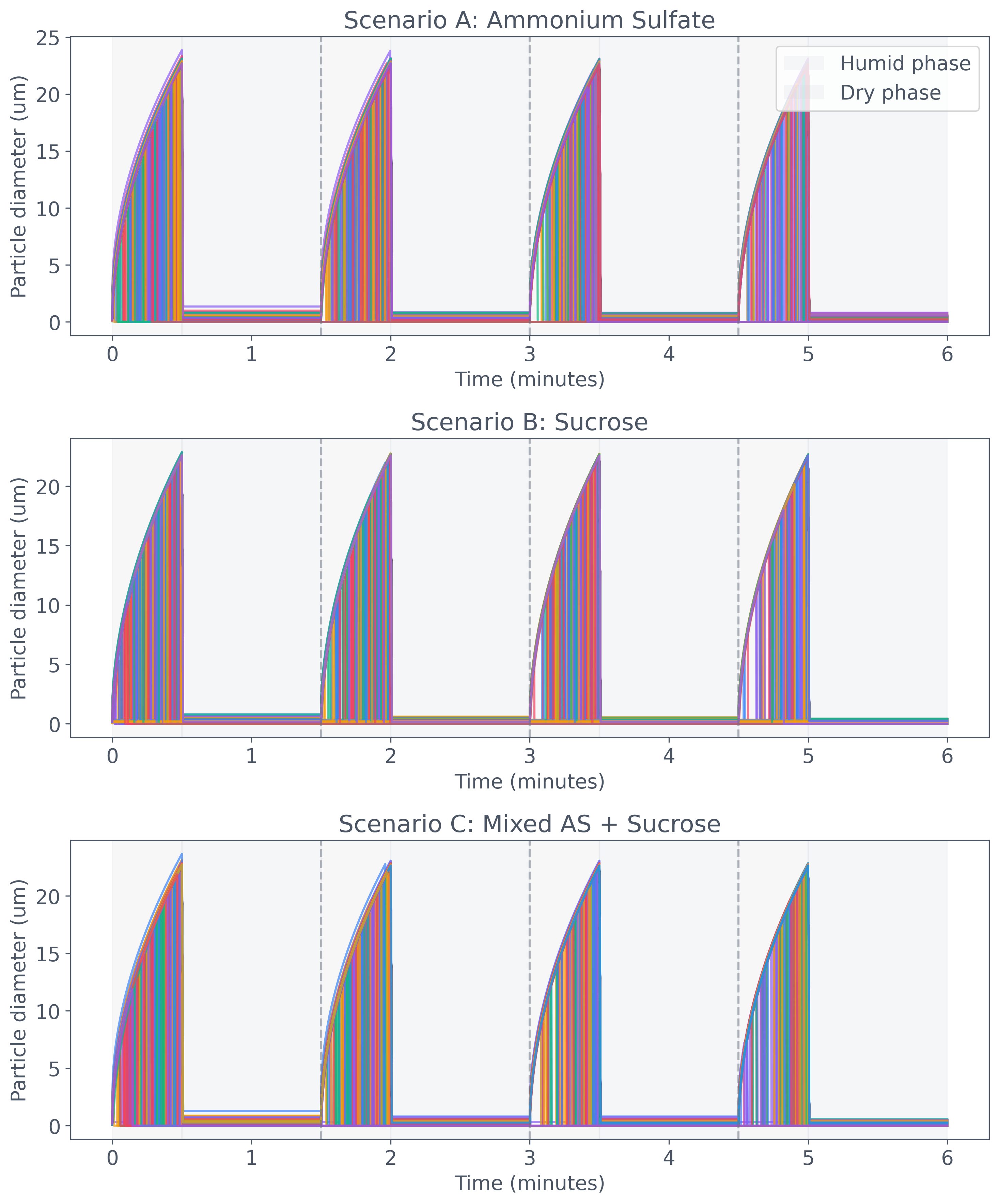
Define the plotted “activated fraction” precisely
Section titled “Define the plotted “activated fraction” precisely”For each original particle slot, count humid-phase records with diameter above 2 µm, then divide by the number of humid records. This is a fraction of sampled humid states, not the fraction of the population activated at one time and not an independently calculated Köhler critical point. Removed slots contribute zero thereafter. The initial dry diameter locates each slot on the horizontal axis.
Python · section 9
def calculate_activated_fraction(    history: list, density_array: np.ndarray, activation_threshold: float = 2e-6) -> np.ndarray:    """Calculate fraction of time each particle spends activated during humid phases.
    Args:        history: Simulation history.        density_array: Density array for diameter calculation.        activation_threshold: Diameter threshold for activation (m).
    Returns:        Activated fraction for each particle.    """    humid_records = [r for r in history if r["phase"] == "humid"]    if len(humid_records) == 0:        return np.zeros(history[0]["masses"].shape[0])
    n_particles = humid_records[0]["masses"].shape[0]    activated_count = np.zeros(n_particles)
    for record in humid_records:        diameters = masses_to_diameter_generic(record["masses"], density_array)        activated_count += (diameters > activation_threshold).astype(float)
    return activated_count / len(humid_records)

# Calculate activated fractions for each scenarioactivated_as = calculate_activated_fraction(history_as, density_as)activated_sucrose = calculate_activated_fraction(    history_sucrose, density_sucrose)activated_mixed = calculate_activated_fraction(history_mixed, density_mixed)
# Get initial dry diameters from history (before water uptake)initial_diams_as = (    masses_to_diameter_generic(history_as[0]["masses"], density_as) * 1e9)  # nminitial_diams_sucrose = (    masses_to_diameter_generic(history_sucrose[0]["masses"], density_sucrose)    * 1e9)  # nminitial_diams_mixed = (    masses_to_diameter_generic(history_mixed[0]["masses"], density_mixed) * 1e9)  # nm
# Create scatter plot of activated fraction vs dry diameterfig, ax = plt.subplots(figsize=(8, 5))
ax.scatter(    initial_diams_as,    activated_as,    color=TAILWIND["blue"]["500"],    s=50,    alpha=0.7,    label="AS only (kappa=0.61)",)ax.scatter(    initial_diams_sucrose,    activated_sucrose,    color=TAILWIND["amber"]["500"],    s=50,    alpha=0.7,    label="Sucrose only (kappa=0.10)",)ax.scatter(    initial_diams_mixed,    activated_mixed,    color=TAILWIND["emerald"]["500"],    s=50,    alpha=0.7,    label="Mixed AS + Sucrose",)
ax.set_xlabel("Initial dry diameter (nm)")ax.set_ylabel("Activated fraction")ax.set_title("Humid-state threshold fraction vs initial dry diameter")ax.set_ylim(-0.05, 1.05)ax.set_xscale("log")ax.legend(loc="lower right")ax.grid(True, alpha=0.3)
plt.tight_layout()plt.show()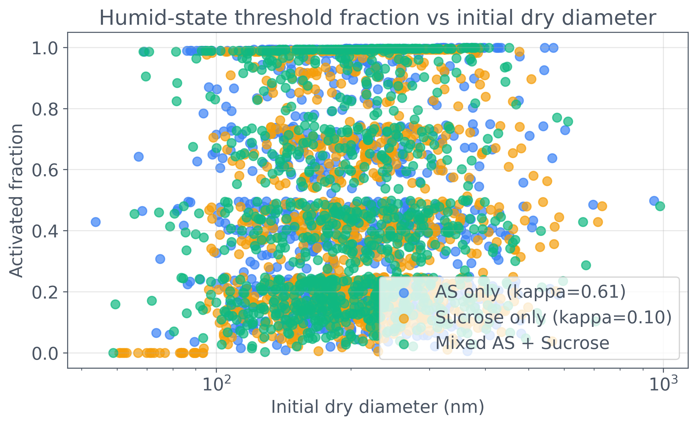
Average water fractions over surviving particles
Section titled “Average water fractions over surviving particles”This panel averages each nonempty particle’s water/total-mass ratio with equal particle weight. It answers a different question from the later bulk water fraction, which divides total water mass by total particle mass. Preferential removal can change either statistic even at similar humidity forcing.
Python · section 10
def calculate_mean_water_fraction(history: list, water_index: int) -> tuple:    """Calculate mean water mass fraction over time.
    Args:        history: Simulation history.        water_index: Index of water species.
    Returns:        Tuple of (times, mean_water_fractions).    """    times = []    water_fractions = []
    for record in history:        masses = record["masses"]        total_mass = masses.sum(axis=1)        water_mass = masses[:, water_index]
        # Avoid division by zero        valid = total_mass > 0        if valid.any():            fractions = np.divide(                water_mass,                total_mass,                out=np.zeros_like(water_mass),                where=valid,            )            mean_frac = fractions[valid].mean()        else:            mean_frac = 0
        times.append(record["time"])        water_fractions.append(mean_frac)
    return np.array(times), np.array(water_fractions)

# Calculate water fractions for each scenariotimes_as, water_frac_as = calculate_mean_water_fraction(    history_as, water_index=1)times_sucrose, water_frac_sucrose = calculate_mean_water_fraction(    history_sucrose, water_index=1)times_mixed, water_frac_mixed = calculate_mean_water_fraction(    history_mixed, water_index=2)
# Create plotfig, ax = plt.subplots(figsize=(10, 5))
# Shade phasesfor cycle in range(n_cycles):    start = cycle * cycle_duration    mid = start + humid_duration    end = start + cycle_duration    ax.axvspan(start / 60, mid / 60, color=TAILWIND["gray"]["200"], alpha=0.3)    ax.axvspan(mid / 60, end / 60, color=TAILWIND["gray"]["300"], alpha=0.2)
ax.plot(    times_as / 60,    water_frac_as,    color=TAILWIND["blue"]["500"],    linewidth=2,    label="AS only (kappa=0.61)",)ax.plot(    times_sucrose / 60,    water_frac_sucrose,    color=TAILWIND["amber"]["500"],    linewidth=2,    label="Sucrose only (kappa=0.10)",)ax.plot(    times_mixed / 60,    water_frac_mixed,    color=TAILWIND["emerald"]["500"],    linewidth=2,    label="Mixed AS + Sucrose",)
ax.set_xlabel("Time (minutes)")ax.set_ylabel("Mean water mass fraction")ax.set_title("Water Mass Fraction Evolution Over 4 Cycles")ax.legend()ax.grid(True, alpha=0.3)
plt.tight_layout()plt.show()
print("Key observations:")print("  - Compare water uptake for these sampled compositions and forcing")print("  - Periodic pattern reflects activation-deactivation cycles")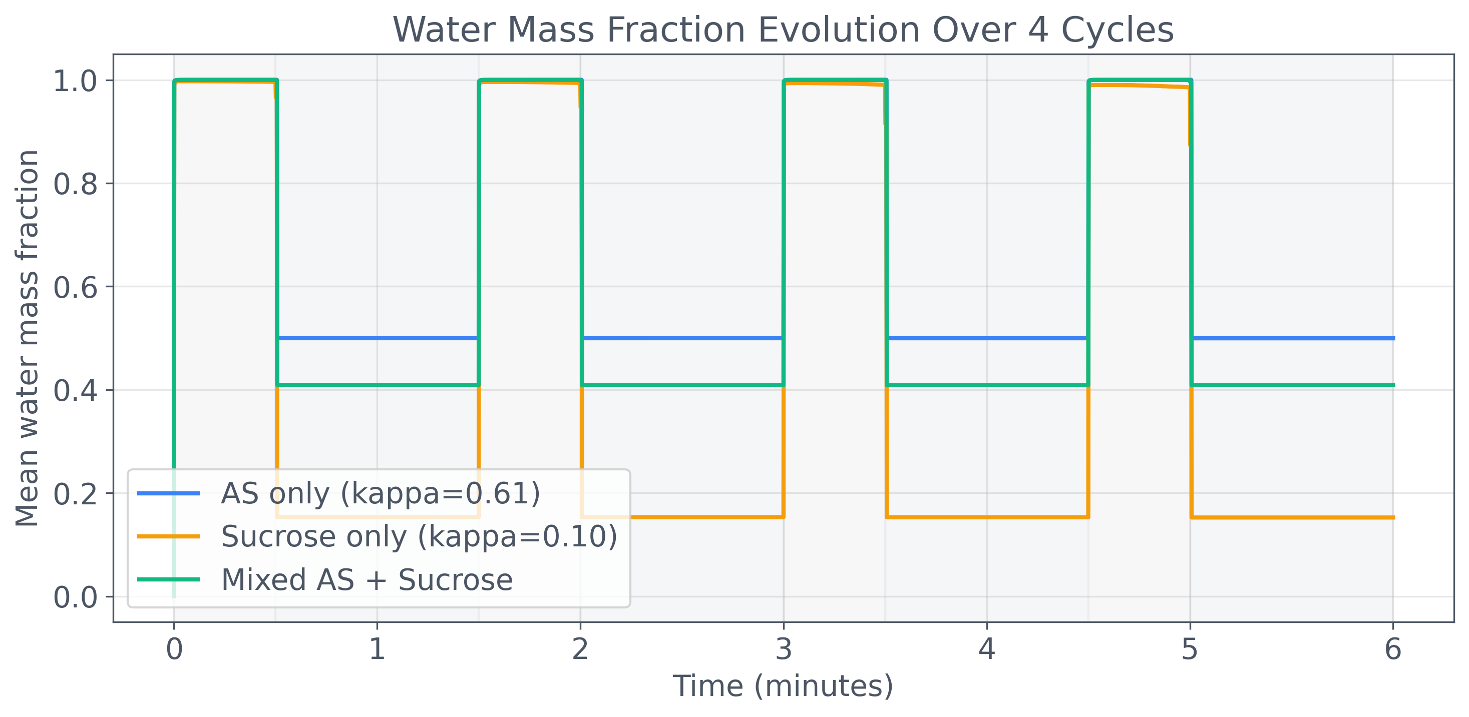
Key observations:
  - Compare water uptake for these sampled compositions and forcing
  - Periodic pattern reflects activation-deactivation cycles
Measure retained dry material after each cycle
Section titled “Measure retained dry material after each cycle”The bars sum all nonwater mass at each cycle end and divide by its initial value. This is whole-population dry-mass retention, not retention in separate size bins. It is not a test of water conservation, because the reservoir is reset repeatedly. Dry removal and wet-mass growth can occur simultaneously.
Python · section 11
def get_total_dry_mass_at_cycle_ends(    history: list, water_index: int, cycle_duration: int) -> tuple:    """Extract total dry mass (non-water) at the end of each cycle.
    Args:        history: Simulation history.        water_index: Index of water species.        cycle_duration: Duration of one cycle in seconds.
    Returns:        Tuple of (cycle_numbers, total_dry_masses).    """    cycle_numbers = []    total_dry_masses = []    for record in history:        # Check if this is end of a cycle (time is multiple of cycle_duration)        if record["time"] > 0 and record["time"] % cycle_duration == 0:            masses = record["masses"]            # Sum all non-water species across all particles            dry_mass = (masses.sum(axis=1) - masses[:, water_index]).sum()            cycle_numbers.append(int(record["time"] / cycle_duration))            total_dry_masses.append(dry_mass)    return cycle_numbers, total_dry_masses

# Get dry mass at cycle endscycles_as, dry_mass_as = get_total_dry_mass_at_cycle_ends(    history_as, water_index=1, cycle_duration=90)cycles_sucrose, dry_mass_sucrose = get_total_dry_mass_at_cycle_ends(    history_sucrose, water_index=1, cycle_duration=90)cycles_mixed, dry_mass_mixed = get_total_dry_mass_at_cycle_ends(    history_mixed, water_index=2, cycle_duration=90)
# Initial dry masses (total across all particles)initial_dry_as = history_as[0]["masses"][:, 0].sum()  # AS massinitial_dry_sucrose = history_sucrose[0]["masses"][:, 0].sum()  # Sucrose massinitial_dry_mixed = (    history_mixed[0]["masses"][:, 0] + history_mixed[0]["masses"][:, 1]).sum()  # AS + Sucrose
# Calculate relative retention (fraction of initial mass remaining)retention_as = [dm / initial_dry_as for dm in dry_mass_as]retention_sucrose = [dm / initial_dry_sucrose for dm in dry_mass_sucrose]retention_mixed = [dm / initial_dry_mixed for dm in dry_mass_mixed]
fig, ax = plt.subplots(figsize=(8, 5))
x = np.arange(1, n_cycles + 1)width = 0.25
ax.bar(    x - width,    retention_as,    width,    label="AS only",    color=TAILWIND["blue"]["500"],)ax.bar(    x,    retention_sucrose,    width,    label="Sucrose only",    color=TAILWIND["amber"]["500"],)ax.bar(    x + width,    retention_mixed,    width,    label="Mixed",    color=TAILWIND["emerald"]["500"],)
ax.set_xlabel("Cycle number")ax.set_ylabel("Dry mass retention fraction")ax.set_title("Dry Mass Retention Over Cycles")ax.set_xticks(x)ax.legend()ax.set_ylim(0, 1.1)ax.grid(True, alpha=0.3, axis="y")
plt.tight_layout()plt.show()
print("Key observations:")print("  - Mass decreases over cycles due to wall loss")print(    "  - Dilution is disabled; humidity resets exchange water with the reservoir")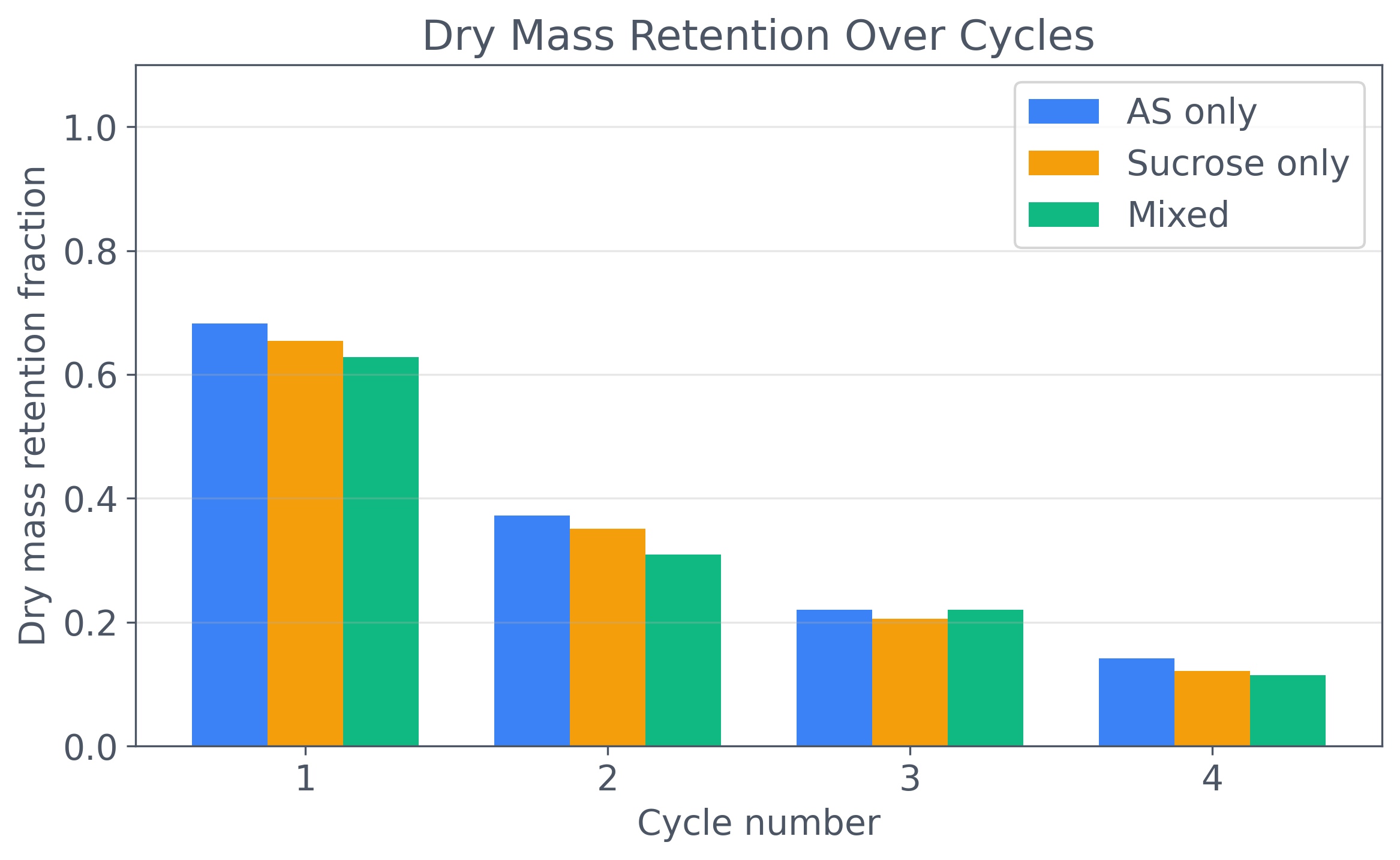
Key observations:
  - Mass decreases over cycles due to wall loss
  - Dilution is disabled; humidity resets exchange water with the reservoir
Compare means without hiding selection effects
Section titled “Compare means without hiding selection effects”The mean-diameter curves include only nonempty particle slots. Water exchange changes their sizes and wall loss changes which particles remain. The curves therefore cannot isolate κ or define an activation ordering without considering the different initial samples, loss histories, and numerical resolution.
Python · section 12
def calculate_mean_diameter(history: list, density_array: np.ndarray) -> tuple:    """Calculate mean particle diameter over time.
    Args:        history: Simulation history.        density_array: Density array for diameter calculation.
    Returns:        Tuple of (times, mean_diameters).    """    times = []    mean_diams = []
    for record in history:        diameters = masses_to_diameter_generic(record["masses"], density_array)        valid = diameters > 0        if valid.any():            mean_d = diameters[valid].mean()        else:            mean_d = 0        times.append(record["time"])        mean_diams.append(mean_d)
    return np.array(times), np.array(mean_diams)

# Calculate mean diameterstimes_as, mean_diam_as = calculate_mean_diameter(history_as, density_as)times_sucrose, mean_diam_sucrose = calculate_mean_diameter(    history_sucrose, density_sucrose)times_mixed, mean_diam_mixed = calculate_mean_diameter(    history_mixed, density_mixed)
# Create overlay plotfig, ax = plt.subplots(figsize=(10, 6))
# Shade phasesfor cycle in range(n_cycles):    start = cycle * cycle_duration    mid = start + humid_duration    end = start + cycle_duration    if cycle == 0:        ax.axvspan(            start / 60,            mid / 60,            color=TAILWIND["sky"]["300"],            alpha=0.3,            label="Humid phase",        )        ax.axvspan(            mid / 60,            end / 60,            color=TAILWIND["gray"]["200"],            alpha=0.2,            label="Dry phase",        )    else:        ax.axvspan(            start / 60, mid / 60, color=TAILWIND["sky"]["300"], alpha=0.3        )        ax.axvspan(mid / 60, end / 60, color=TAILWIND["gray"]["200"], alpha=0.2)
ax.plot(    times_as / 60,    mean_diam_as * 1e6,    color=TAILWIND["blue"]["700"],    linewidth=2.5,    label="AS only (kappa=0.61)",)ax.plot(    times_sucrose / 60,    mean_diam_sucrose * 1e6,    color=TAILWIND["amber"]["600"],    linewidth=2.5,    label="Sucrose only (kappa=0.10)",)ax.plot(    times_mixed / 60,    mean_diam_mixed * 1e6,    color=TAILWIND["teal"]["500"],    linewidth=2.5,    label="Mixed AS + Sucrose",)
ax.set_xlabel("Time (minutes)")ax.set_ylabel("Mean particle diameter (um)")ax.set_title("Mean wet size across three sampled compositions")ax.legend(loc="upper right")ax.grid(True, alpha=0.3)
plt.tight_layout()plt.show()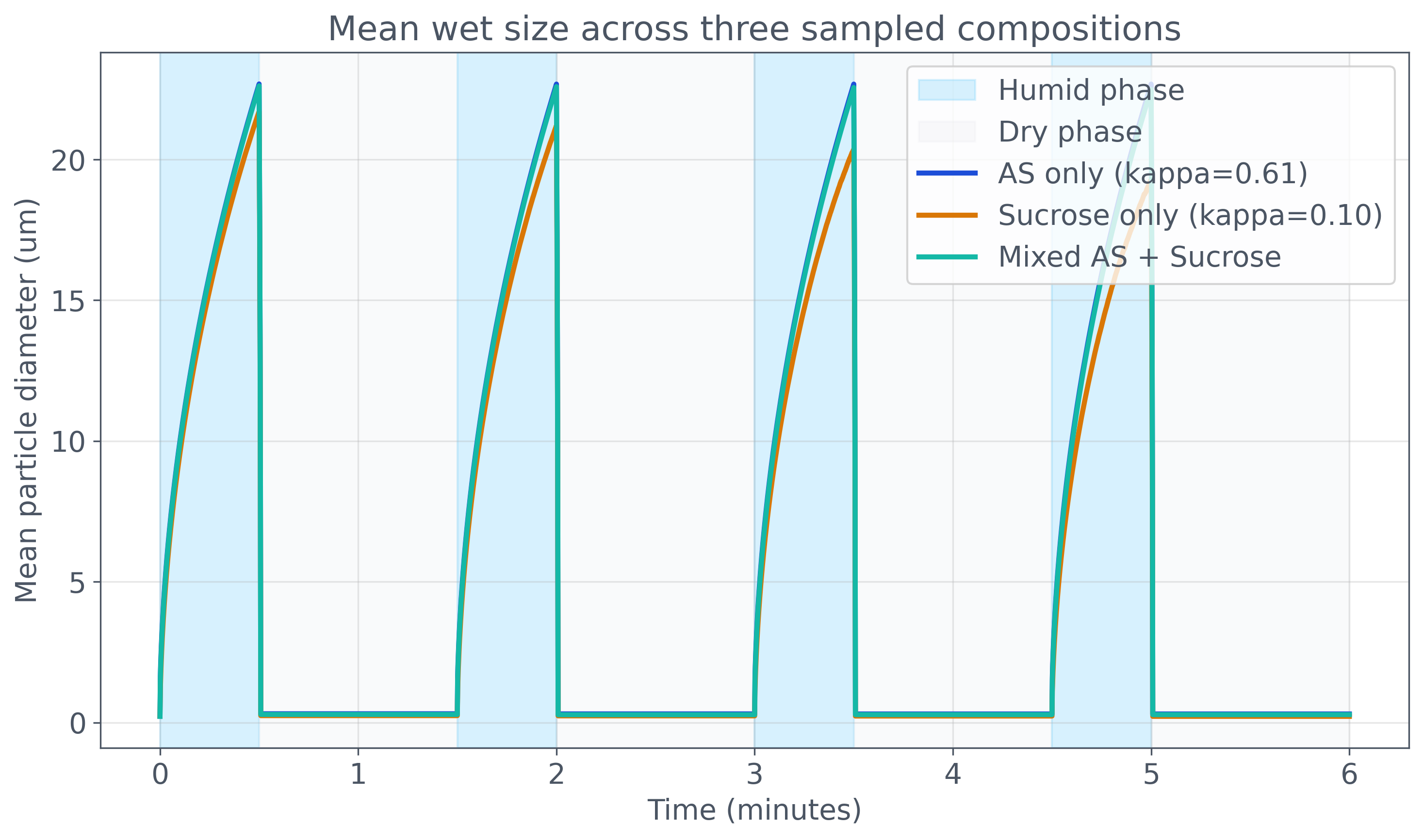
Interpret each check at the scope it actually tests
Section titled “Interpret each check at the scope it actually tests”The checks cover the standalone dilution formula, history structure, species widths, finite nonnegative masses, cycle count, and selected threshold timings. They use several different definitions: the scatter uses 2 µm, the first-event check uses 1 µm, and the per-particle check uses twice initial diameter. These are diagnostics, not interchangeable definitions of critical activation.
The adjacent-slot timing assertion retains a 5 s bound and does not sort the sample by size; it cannot establish a monotonic size-dependent activation law. Likewise, passing the sulfate-versus-sucrose first-event comparison is evidence for this realization only. The printed “all checks passed” is not physical validation. Closed condensation inventories were checked separately inside the integration loop; a final wet/dry mass ratio is not their error measure.
Python · section 13
# 18.1 Validate apply_count_dilution() produces expected decaytest_counts = np.array([1.0, 2.0, 3.0, 4.0])  # represented countsdiluted = apply_count_dilution(test_counts, dilution_coefficient=0.01, dt=1.0)expected_factor = np.exp(-0.01 * 1.0)  # ~0.99005assert np.allclose(diluted, test_counts * expected_factor), (    "Dilution decay incorrect")assert np.all(diluted > 0), "Dilution should preserve positive counts"assert np.all(diluted < test_counts), "Dilution should reduce counts"print("1. apply_count_dilution() validated")

# 18.2 Validate history structuredef validate_history(history, name, n_cycles, cycle_duration):    """Validate history records from simulation."""    assert len(history) > 0, f"{name}: History is empty"
    # Check all records have required keys    required_keys = {"time", "phase", "masses"}    for i, record in enumerate(history):        assert required_keys.issubset(record.keys()), (            f"{name}: Record {i} missing keys"        )
    # Check time progression    times = [r["time"] for r in history]    assert times == sorted(times), f"{name}: Times not monotonically increasing"
    # Check final time approximately matches expected duration    expected_duration = n_cycles * cycle_duration    assert abs(times[-1] - expected_duration) < cycle_duration, (        f"{name}: Final time mismatch"    )
    # Check phases alternate (humid, dry)    phases = [r["phase"] for r in history]    assert set(phases) == {"humid", "dry"}, f"{name}: Unexpected phase values"
    print(        f"2. {name} history validated ({len(history)} records, {times[-1]:.0f}s)"    )

validate_history(history_as, "AS", n_cycles=4, cycle_duration=90)validate_history(history_sucrose, "Sucrose", n_cycles=4, cycle_duration=90)validate_history(history_mixed, "Mixed", n_cycles=4, cycle_duration=90)
# 18.3 Validate scenario setup (species count and shapes)as_first_masses = history_as[0]["masses"]assert as_first_masses.shape[1] == 2, "AS should have 2 species (AS, water)"print(    f"3. AS scenario: {as_first_masses.shape[0]} particles, "    f"{as_first_masses.shape[1]} species")
sucrose_first_masses = history_sucrose[0]["masses"]assert sucrose_first_masses.shape[1] == 2, "Sucrose should have 2 species"print(    f"   Sucrose scenario: {sucrose_first_masses.shape[0]} particles, "    f"{sucrose_first_masses.shape[1]} species")
mixed_first_masses = history_mixed[0]["masses"]assert mixed_first_masses.shape[1] == 3, (    "Mixed should have 3 species (AS, sucrose, water)")assert mixed_first_masses.shape[0] == n_particles_mixed, (    f"Mixed should have {n_particles_mixed} particles")print(    f"   Mixed scenario: {mixed_first_masses.shape[0]} particles, "    f"{mixed_first_masses.shape[1]} species")
1. apply_count_dilution() validated
2. AS history validated (3601 records, 360s)
2. Sucrose history validated (3601 records, 360s)
2. Mixed history validated (3601 records, 360s)
3. AS scenario: 1000 particles, 2 species
Sucrose scenario: 1000 particles, 2 species
Mixed scenario: 1000 particles, 3 speciesPython · section 14
# 18.4 Validate kappa-dependent activation orderdef get_first_activation_time(    history, density_array, threshold_diameter_m=1e-6):    """Get time when any particle first exceeds threshold diameter."""    for record in history:        diameters = masses_to_diameter_generic(record["masses"], density_array)        if np.any(diameters > threshold_diameter_m):            return record["time"]    return float("inf")  # Never activated

as_activation_time = get_first_activation_time(history_as, density_as)sucrose_activation_time = get_first_activation_time(    history_sucrose, density_sucrose)
print("4. kappa-dependent activation:")print(f"   AS first activation: {as_activation_time}s")print(f"   Sucrose first activation: {sucrose_activation_time}s")
# AS should activate at same time or before sucrose (higher kappa)assert as_activation_time <= sucrose_activation_time, (    f"AS (kappa=0.61) should activate before or with sucrose (kappa=0.10): "    f"AS at {as_activation_time}s, sucrose at {sucrose_activation_time}s")print("   Validated: AS activates at same time or before sucrose")

# 18.5 Validate size-dependent activation (larger particles activate earlier)def get_activation_times_by_particle(    history, density_array, threshold_factor=2.0):    """Get activation time for each particle.
    Activation defined as diameter > threshold_factor * initial diameter.    """    initial_diameters = masses_to_diameter_generic(        history[0]["masses"], density_array    )    thresholds = initial_diameters * threshold_factor    n_particles = len(initial_diameters)    activation_times = np.full(n_particles, float("inf"))
    for record in history:        diameters = masses_to_diameter_generic(record["masses"], density_array)        newly_activated = (diameters > thresholds) & (            activation_times == float("inf")        )        activation_times[newly_activated] = record["time"]
    return activation_times, initial_diameters

as_act_times, as_initial_diams = get_activation_times_by_particle(    history_as, density_as)
print("5. Size-dependent activation for AS scenario:")print(f"   Dry diameters (nm): {(as_initial_diams * 1e9).astype(int)}")print(f"   Activation times (s): {as_act_times}")
# Verify trend: larger particles (higher index) activate earlier or at same time# Allow 5s tolerance for simulation artifactsfor i in range(len(as_act_times) - 1):    if as_act_times[i] < float("inf") and as_act_times[i + 1] < float("inf"):        assert as_act_times[i] >= as_act_times[i + 1] - 5, (            f"Size-dependent activation violated: particle {i} "            f"(d={as_initial_diams[i] * 1e9:.0f}nm) "            f"activated at {as_act_times[i]}s but particle {i + 1} "            f"(d={as_initial_diams[i + 1] * 1e9:.0f}nm) "            f"activated at {as_act_times[i + 1]}s"        )
print("   Adjacent-slot activation-time check passed within its 5 s bound")
4. kappa-dependent activation:
AS first activation: 0.1s
Sucrose first activation: 0.1s
Validated: AS activates at same time or before sucrose
5. Size-dependent activation for AS scenario:
Dry diameters (nm): [244 189 260 370 181 181 379 273 165 249 165 165 220 92 99 159 132 227
138 112 362 182 205 112 160 209 125 232 156 177 156 423 198 130 279 121
217 90 116 216 269 214 190 177 109 149 165 307 229 97 228 171 151 256
303 291 142 176 228 297 164 185 127 123 278 346 194 300 231 153 231 373
197 377 69 279 207 177 207 89 182 231 364 162 144 163 289 228 161 246
208 296 150 175 170 110 225 222 200 181 112 168 174 144 187 235 429 214
222 194 91 197 204 542 184 226 197 124 317 271 275 138 353 113 253 486
133 158 208 163 106 205 130 242 137 374 145 175 278 121 219 339 104 215
222 274 121 117 247 225 221 230 151 219 225 149 426 242 123 261 134 275
319 143 295 236 279 431 181 147 139 143 193 229 223 279 201 360 179 602
257 141 129 243 182 267 242 194 141 108 166 283 218 120 214 233 139 212
204 125 231 251 310 306 114 136 246 246 246 953 252 316 294 260 176 272
146 181 164 206 511 93 264 104 165 311 205 129 149 263 148 218 203 153
477 258 87 215 152 282 145 190 245 284 122 174 164 153 409 235 119 290
472 303 108 164 334 150 239 273 137 195 53 132 180 120 387 111 167 210
358 111 320 200 134 241 216 156 205 171 209 261 380 121 474 90 188 253
224 155 183 163 157 282 231 151 288 226 278 258 142 159 270 256 198 209
335 157 249 184 183 312 279 278 339 201 263 176 228 189 208 254 143 467
133 122 319 275 257 258 199 139 206 151 296 188 143 175 236 159 143 220
220 162 165 219 111 113 149 183 226 363 283 187 198 133 198 177 227 143
246 372 191 235 264 169 219 201 208 146 201 244 360 295 478 146 284 215
485 144 142 156 84 161 147 212 229 427 294 158 138 244 117 420 322 165
99 346 190 330 104 156 200 203 166 257 129 188 209 246 266 126 107 335
228 147 375 209 322 205 461 407 180 296 259 348 135 264 307 98 123 87
179 267 367 206 387 114 100 195 233 197 86 192 117 262 232 136 162 130
194 294 134 245 161 145 191 131 159 123 443 202 150 218 191 182 256 271
161 158 178 78 108 348 389 180 252 226 696 314 189 135 104 217 147 112
153 128 396 285 199 364 206 141 370 248 131 185 140 114 291 433 113 251
153 164 157 140 203 142 223 195 181 138 158 271 245 134 208 271 101 249
152 252 146 96 103 203 222 138 259 101 194 122 153 203 141 171 300 158
280 126 247 358 73 144 252 184 232 156 207 187 321 221 229 169 164 167
234 168 224 463 284 175 325 169 87 132 93 173 201 394 228 182 279 81
220 273 109 318 229 169 258 502 215 221 166 141 280 141 205 164 242 228
304 162 179 134 167 233 271 137 284 346 236 428 146 120 97 366 260 195
224 126 539 210 209 268 243 219 145 242 428 345 381 162 133 190 204 311
100 371 187 168 132 102 279 206 118 118 174 393 180 108 181 179 67 195
182 265 423 315 179 127 567 204 201 198 216 188 158 160 197 160 149 208
180 368 68 311 331 86 174 172 113 145 127 406 292 334 267 126 161 243
121 267 181 171 266 239 172 320 129 256 254 176 228 120 290 185 161 306
150 112 106 255 119 407 85 397 217 192 160 235 196 312 209 212 172 195
226 99 115 270 214 185 201 230 160 145 216 134 236 100 303 242 221 297
392 301 94 119 155 202 246 149 215 147 156 113 137 115 134 306 136 581
244 215 141 265 158 210 564 192 318 150 197 410 155 417 266 159 258 296
257 105 148 180 194 257 214 116 233 256 250 309 280 240 194 101 238 217
223 119 129 306 196 263 202 202 292 162 207 165 167 176 218 164 332 139
185 167 359 216 303 109 222 286 206 308 162 354 507 172 166 360 379 161
168 178 115 137 133 146 197 219 375 133 298 183 196 262 126 233 213 244
224 541 154 161 155 159 154 323 355 158 142 242 159 258 217 108 374 414
155 170 224 229 261 451 186 144 114 148 197 414 162 218 198 323 557 161
164 305 263 422 253 172 254 313 278 245 308 321 350 260 186 212 326 143
232 170 202 335 216 203 115 270 259 480 176 218 221 379 192 223 255 215
166 216 309 131 211 150 324 107 159 233 377 194 159 428 111 82 239 163
132 266 220 159 119 284 260 192 422 129 107 151 196 220 181 230 120 359
193 314 229 240 251 239 259 342 216 266 192 358 152 415 196 111 210 151
281 153 166 92 166 74 105 272 275 237 135 196 199 125 367 285 182 202
217 87 180 151 133 178 414 259 158 252]
Activation times (s): [0.1 0.1 0.1 0.1 0.1 0.1 0.1 0.1 0.1 0.1 0.1 0.1 0.1 0.1 0.1 0.1 0.1 0.1
0.1 0.1 0.1 0.1 0.1 0.1 0.1 0.1 0.1 0.1 0.1 0.1 0.1 0.1 0.1 0.1 0.1 0.1
0.1 0.1 0.1 0.1 0.1 0.1 0.1 0.1 0.1 0.1 0.1 0.1 0.1 0.1 0.1 0.1 0.1 0.1
0.1 0.1 0.1 0.1 0.1 0.1 0.1 0.1 0.1 0.1 0.1 0.1 0.1 0.1 0.1 0.1 0.1 0.1
0.1 0.1 0.1 0.1 0.1 0.1 0.1 0.1 0.1 0.1 0.1 0.1 0.1 0.1 0.1 0.1 0.1 0.1
0.1 0.1 0.1 0.1 0.1 0.1 0.1 0.1 0.1 0.1 0.1 0.1 0.1 0.1 0.1 0.1 0.1 0.1
0.1 0.1 0.1 0.1 0.1 0.1 0.1 0.1 0.1 0.1 0.1 0.1 0.1 0.1 0.1 0.1 0.1 0.1
0.1 0.1 0.1 0.1 0.1 0.1 0.1 0.1 0.1 0.1 0.1 0.1 0.1 0.1 0.1 0.1 0.1 0.1
0.1 0.1 0.1 0.1 0.1 0.1 0.1 0.1 0.1 0.1 0.1 0.1 0.1 0.1 0.1 0.1 0.1 0.1
0.1 0.1 0.1 0.1 0.1 0.1 0.1 0.1 0.1 0.1 0.1 0.1 0.1 0.1 0.1 0.1 0.1 0.1
0.1 0.1 0.1 0.1 0.1 0.1 0.1 0.1 0.1 0.1 0.1 0.1 0.1 0.1 0.1 0.1 0.1 0.1
0.1 0.1 0.1 0.1 0.1 0.1 0.1 0.1 0.1 0.1 0.1 0.1 0.1 0.1 0.1 0.1 0.1 0.1
0.1 0.1 0.1 0.1 0.1 0.1 0.1 0.1 0.1 0.1 0.1 0.1 0.1 0.1 0.1 0.1 0.1 0.1
0.1 0.1 0.1 0.1 0.1 0.1 0.1 0.1 0.1 0.1 0.1 0.1 0.1 0.1 0.1 0.1 0.1 0.1
0.1 0.1 0.1 0.1 0.1 0.1 0.1 0.1 0.1 0.1 0.1 0.1 0.1 0.1 0.1 0.1 0.1 0.1
0.1 0.1 0.1 0.1 0.1 0.1 0.1 0.1 0.1 0.1 0.1 0.1 0.1 0.1 0.1 0.1 0.1 0.1
0.1 0.1 0.1 0.1 0.1 0.1 0.1 0.1 0.1 0.1 0.1 0.1 0.1 0.1 0.1 0.1 0.1 0.1
0.1 0.1 0.1 0.1 0.1 0.1 0.1 0.1 0.1 0.1 0.1 0.1 0.1 0.1 0.1 0.1 0.1 0.1
0.1 0.1 0.1 0.1 0.1 0.1 0.1 0.1 0.1 0.1 0.1 0.1 0.1 0.1 0.1 0.1 0.1 0.1
0.1 0.1 0.1 0.1 0.1 0.1 0.1 0.1 0.1 0.1 0.1 0.1 0.1 0.1 0.1 0.1 0.1 0.1
0.1 0.1 0.1 0.1 0.1 0.1 0.1 0.1 0.1 0.1 0.1 0.1 0.1 0.1 0.1 0.1 0.1 0.1
0.1 0.1 0.1 0.1 0.1 0.1 0.1 0.1 0.1 0.1 0.1 0.1 0.1 0.1 0.1 0.1 0.1 0.1
0.1 0.1 0.1 0.1 0.1 0.1 0.1 0.1 0.1 0.1 0.1 0.1 0.1 0.1 0.1 0.1 0.1 0.1
0.1 0.1 0.1 0.1 0.1 0.1 0.1 0.1 0.1 0.1 0.1 0.1 0.1 0.1 0.1 0.1 0.1 0.1
0.1 0.1 0.1 0.1 0.1 0.1 0.1 0.1 0.1 0.1 0.1 0.1 0.1 0.1 0.1 0.1 0.1 0.1
0.1 0.1 0.1 0.1 0.1 0.1 0.1 0.1 0.1 0.1 0.1 0.1 0.1 0.1 0.1 0.1 0.1 0.1
0.1 0.1 0.1 0.1 0.1 0.1 0.1 0.1 0.1 0.1 0.1 0.1 0.1 0.1 0.1 0.1 0.1 0.1
0.1 0.1 0.1 0.1 0.1 0.1 0.1 0.1 0.1 0.1 0.1 0.1 0.1 0.1 0.1 0.1 0.1 0.1
0.1 0.1 0.1 0.1 0.1 0.1 0.1 0.1 0.1 0.1 0.1 0.1 0.1 0.1 0.1 0.1 0.1 0.1
0.1 0.1 0.1 0.1 0.1 0.1 0.1 0.1 0.1 0.1 0.1 0.1 0.1 0.1 0.1 0.1 0.1 0.1
0.1 0.1 0.1 0.1 0.1 0.1 0.1 0.1 0.1 0.1 0.1 0.1 0.1 0.1 0.1 0.1 0.1 0.1
0.1 0.1 0.1 0.1 0.1 0.1 0.1 0.1 0.1 0.1 0.1 0.1 0.1 0.1 0.1 0.1 0.1 0.1
0.1 0.1 0.1 0.1 0.1 0.1 0.1 0.1 0.1 0.1 0.1 0.1 0.1 0.1 0.1 0.1 0.1 0.1
0.1 0.1 0.1 0.1 0.1 0.1 0.1 0.1 0.1 0.1 0.1 0.1 0.1 0.1 0.1 0.1 0.1 0.1
0.1 0.1 0.1 0.1 0.1 0.1 0.1 0.1 0.1 0.1 0.1 0.1 0.1 0.1 0.1 0.1 0.1 0.1
0.1 0.1 0.1 0.1 0.1 0.1 0.1 0.1 0.1 0.1 0.1 0.1 0.1 0.1 0.1 0.1 0.1 0.1
0.1 0.1 0.1 0.1 0.1 0.1 0.1 0.1 0.1 0.1 0.1 0.1 0.1 0.1 0.1 0.1 0.1 0.1
0.1 0.1 0.1 0.1 0.1 0.1 0.1 0.1 0.1 0.1 0.1 0.1 0.1 0.1 0.1 0.1 0.1 0.1
0.1 0.1 0.1 0.1 0.1 0.1 0.1 0.1 0.1 0.1 0.1 0.1 0.1 0.1 0.1 0.1 0.1 0.1
0.1 0.1 0.1 0.1 0.1 0.1 0.1 0.1 0.1 0.1 0.1 0.1 0.1 0.1 0.1 0.1 0.1 0.1
0.1 0.1 0.1 0.1 0.1 0.1 0.1 0.1 0.1 0.1 0.1 0.1 0.1 0.1 0.1 0.1 0.1 0.1
0.1 0.1 0.1 0.1 0.1 0.1 0.1 0.1 0.1 0.1 0.1 0.1 0.1 0.1 0.1 0.1 0.1 0.1
0.1 0.1 0.1 0.1 0.1 0.1 0.1 0.1 0.1 0.1 0.1 0.1 0.1 0.1 0.1 0.1 0.1 0.1
0.1 0.1 0.1 0.1 0.1 0.1 0.1 0.1 0.1 0.1 0.1 0.1 0.1 0.1 0.1 0.1 0.1 0.1
0.1 0.1 0.1 0.1 0.1 0.1 0.1 0.1 0.1 0.1 0.1 0.1 0.1 0.1 0.1 0.1 0.1 0.1
0.1 0.1 0.1 0.1 0.1 0.1 0.1 0.1 0.1 0.1 0.1 0.1 0.1 0.1 0.1 0.1 0.1 0.1
0.1 0.1 0.1 0.1 0.1 0.1 0.1 0.1 0.1 0.1 0.1 0.1 0.1 0.1 0.1 0.1 0.1 0.1
0.1 0.1 0.1 0.1 0.1 0.1 0.1 0.1 0.1 0.1 0.1 0.1 0.1 0.1 0.1 0.1 0.1 0.1
0.1 0.1 0.1 0.1 0.1 0.1 0.1 0.1 0.1 0.1 0.1 0.1 0.1 0.1 0.1 0.1 0.1 0.1
0.1 0.1 0.1 0.1 0.1 0.1 0.1 0.1 0.1 0.1 0.1 0.1 0.1 0.1 0.1 0.1 0.1 0.1
0.1 0.1 0.1 0.1 0.1 0.1 0.1 0.1 0.1 0.1 0.1 0.1 0.1 0.1 0.1 0.1 0.1 0.1
0.1 0.1 0.1 0.1 0.1 0.1 0.1 0.1 0.1 0.1 0.1 0.1 0.1 0.1 0.1 0.1 0.1 0.1
0.1 0.1 0.1 0.1 0.1 0.1 0.1 0.1 0.1 0.1 0.1 0.1 0.1 0.1 0.1 0.1 0.1 0.1
0.1 0.1 0.1 0.1 0.1 0.1 0.1 0.1 0.1 0.1 0.1 0.1 0.1 0.1 0.1 0.1 0.1 0.1
0.1 0.1 0.1 0.1 0.1 0.1 0.1 0.1 0.1 0.1 0.1 0.1 0.1 0.1 0.1 0.1 0.1 0.1
0.1 0.1 0.1 0.1 0.1 0.1 0.1 0.1 0.1 0.1]
Adjacent-slot activation-time check passed within its 5 s boundPython · section 15
# 18.6 Validate mass accounting (positive counts, finite values)def calculate_total_mass(masses):    """Calculate total mass across all particles and species."""    return np.sum(masses)

print("6. Mass accounting:")for name, history, water_idx in [    ("AS", history_as, 1),    ("Sucrose", history_sucrose, 1),    ("Mixed", history_mixed, 2),]:    initial_mass = calculate_total_mass(history[0]["masses"])    final_mass = calculate_total_mass(history[-1]["masses"])    # Dry mass (non-water) should decrease due to wall loss    initial_dry = (        history[0]["masses"].sum() - history[0]["masses"][:, water_idx].sum()    )    final_dry = (        history[-1]["masses"].sum() - history[-1]["masses"][:, water_idx].sum()    )
    assert final_mass > 0, f"{name}: Final mass should be positive"    assert final_dry > 0, f"{name}: Final dry mass should be positive"
    mass_change = final_mass / initial_mass    dry_change = final_dry / initial_dry if initial_dry > 0 else 1.0
    print(        f"   {name}: Total {initial_mass:.2e} -> {final_mass:.2e} kg ({mass_change:.1%}), "        f"Dry {initial_dry:.2e} -> {final_dry:.2e} kg ({dry_change:.1%})"    )

# 18.7 Validate all values finite and non-negativedef validate_finite_nonnegative(history, name):    """Check all mass values are finite and non-negative."""    for i, record in enumerate(history):        masses = record["masses"]        assert np.all(np.isfinite(masses)), (            f"{name}: Non-finite masses at record {i}"        )        assert np.all(masses >= 0), f"{name}: Negative masses at record {i}"    print(f"7. {name}: All values finite and non-negative")

validate_finite_nonnegative(history_as, "AS")validate_finite_nonnegative(history_sucrose, "Sucrose")validate_finite_nonnegative(history_mixed, "Mixed")

# 18.8 Validate cycle countdef count_cycles(history, cycle_duration=90):    """Count number of complete cycles based on time span."""    if len(history) == 0:        return 0    total_time = history[-1]["time"]    return int(total_time / cycle_duration)

print("8. Cycle count:")for name, history in [    ("AS", history_as),    ("Sucrose", history_sucrose),    ("Mixed", history_mixed),]:    cycles = count_cycles(history)    assert cycles >= 4, f"{name}: Expected 4 cycles, found {cycles}"    print(f"   {name}: {cycles} cycles completed")
6. Mass accounting:
AS: Total 1.61e-14 -> 4.57e-15 kg (28.4%), Dry 1.61e-14 -> 2.27e-15 kg (14.1%)
Sucrose: Total 1.49e-14 -> 2.13e-15 kg (14.3%), Dry 1.49e-14 -> 1.80e-15 kg (12.1%)
Mixed: Total 1.53e-14 -> 2.98e-15 kg (19.5%), Dry 1.53e-14 -> 1.75e-15 kg (11.5%)7. AS: All values finite and non-negative7. Sucrose: All values finite and non-negative
7. Mixed: All values finite and non-negative
8. Cycle count:
AS: 4 cycles completed
Sucrose: 4 cycles completed
Mixed: 4 cycles completedPython · section 16
# 18.9 Water mass fraction validationdef get_water_fraction_at_phase_peaks(    history, water_index, humid_duration=30, dry_duration=60):    """Get mean water mass fraction at end of each humid phase."""    fractions = []    # Select the last humid record before each dry phase. This also handles    # the initial record and repeated boundary times between cycles.    for record, next_record in zip(history, history[1:]):        if record["phase"] == "humid" and next_record["phase"] == "dry":            masses = record["masses"]            water_mass = masses[:, water_index].sum()            total_mass = masses.sum()            fractions.append(water_mass / total_mass if total_mass > 0 else 0)    return fractions

as_water_fracs = get_water_fraction_at_phase_peaks(    history_as, water_index=1, humid_duration=30, dry_duration=60)sucrose_water_fracs = get_water_fraction_at_phase_peaks(    history_sucrose, water_index=1, humid_duration=30, dry_duration=60)
assert len(as_water_fracs) == len(sucrose_water_fracs) == n_cyclesprint("9. Water mass fraction at humid phase peaks:")if len(as_water_fracs) > 0 and len(sucrose_water_fracs) > 0:    as_mean_water = np.mean(as_water_fracs)    sucrose_mean_water = np.mean(sucrose_water_fracs)    print(f"   AS mean water fraction: {as_mean_water:.3f}")    print(f"   Sucrose mean water fraction: {sucrose_mean_water:.3f}")else:    print("   Insufficient data for water fraction analysis")
# 18.10 Print validation summaryprint("\n" + "=" * 60)print("VALIDATION SUMMARY: ALL CHECKS PASSED")print("=" * 60)print("- Dilution function: Correct exponential decay")print("- History structure: Valid for all 3 scenarios")print("- Scenario setup: Correct species counts and water indices")print(    "- kappa-dependent activation: AS activates at same time or before sucrose")print("- Adjacent-slot activation times pass the retained 5 s bound")print(    "- Closed condensation conserves mapped inventory; wall deposition removes particles")print("- Value validity: All finite and non-negative")print("- Cycle count: 4 cycles completed for each scenario")print("=" * 60)
9. Water mass fraction at humid phase peaks:
AS mean water fraction: 1.000
Sucrose mean water fraction: 1.000
============================================================
VALIDATION SUMMARY: ALL CHECKS PASSED
============================================================
- Dilution function: Correct exponential decay
- History structure: Valid for all 3 scenarios
- Scenario setup: Correct species counts and water indices
- kappa-dependent activation: AS activates at same time or before sucrose
- Adjacent-slot activation times pass the retained 5 s bound
- Closed condensation conserves mapped inventory; wall deposition removes particles
- Value validity: All finite and non-negative
- Cycle count: 4 cycles completed for each scenario
============================================================Compare instantaneous loss coefficients with accumulated removal
Section titled “Compare instantaneous loss coefficients with accumulated removal”The left panel evaluates a reference coefficient at density 1000 kg/m³ over 40–800 nm diameter. The right panel bins initial dry seed mass by initial dry diameter and measures the fraction belonging to slots removed by the end. It is mass-weighted, not a lost-number fraction. Empty initial bins are reported as zero and contain no evidence of low loss.
Wet particles evolve outside those initial dry sizes, so the reference coefficient curve is not their full loss history. The accumulated bars combine growth, drying, and stochastic removal.
Keep chamber removal distinct from water exchange
Section titled “Keep chamber removal distinct from water exchange”Wall loss removes entire resolved particles and their dry material. Evaporation returns water to the modeled gas reservoir; it is not wall deposition. Humidity resets also add or remove water externally. Those processes need separate budgets when comparing with a chamber measurement. This example does not add a wall-desorption or deposited-water reservoir.
Python · section 17
def cumulative_loss_by_bin(history, density_array, bins):    initial_masses = history[0]["masses"]    final_masses = history[-1]["masses"]    initial_diam = masses_to_diameter_generic(initial_masses, density_array)    # Track removed original particle identities. Water uptake changes wet    # sizes, so subtracting wet size-bin totals would not measure deposition.    dry_mass = initial_masses[:, :-1].sum(axis=1)    lost = final_masses.sum(axis=1) == 0    init_bin, _ = np.histogram(initial_diam, bins=bins, weights=dry_mass)    loss_bin, _ = np.histogram(        initial_diam[lost], bins=bins, weights=dry_mass[lost]    )    loss_fraction = np.zeros_like(loss_bin)    mask = init_bin > 0    loss_fraction[mask] = loss_bin[mask] / init_bin[mask]    return loss_bin, loss_fraction

bins = np.geomspace(40e-9, 800e-9, 9)loss_as, loss_frac_as = cumulative_loss_by_bin(history_as, density_as, bins)loss_su, loss_frac_su = cumulative_loss_by_bin(    history_sucrose, density_sucrose, bins)loss_mx, loss_frac_mx = cumulative_loss_by_bin(    history_mixed, density_mixed, bins)
diam_centers = np.sqrt(bins[:-1] * bins[1:]) * 1e9  # nm
# Wall-loss coefficient vs diameter (reuse strategy)diam_grid = np.geomspace(40e-9, 800e-9, 50)radius_grid = diam_grid / 2density_grid = np.full_like(radius_grid, 1000.0)coeff_grid = wall_loss_strategy.loss_coefficient_for_particles(    particle_radius=radius_grid,    particle_density=density_grid,    temperature=temperature,    pressure=total_pressure,)coeff_grid = np.clip(coeff_grid, 0, None)
fig, axes = plt.subplots(1, 2, figsize=(10, 4))
axes[0].semilogx(    diam_grid * 1e9, coeff_grid, color=TAILWIND["blue"]["600"], linewidth=2)axes[0].set_xlabel("Particle diameter (nm)")axes[0].set_ylabel("Wall loss coefficient (1/s)")axes[0].set_title("Rectangular chamber wall loss coefficient")axes[0].grid(True, which="both", alpha=0.3)
width = 0.08 * diam_centersaxes[1].bar(    diam_centers - width,    loss_frac_as,    width,    label="AS",    color=TAILWIND["blue"]["500"],)axes[1].bar(    diam_centers,    loss_frac_su,    width,    label="Sucrose",    color=TAILWIND["amber"]["500"],)axes[1].bar(    diam_centers + width,    loss_frac_mx,    width,    label="Mixed",    color=TAILWIND["emerald"]["500"],)axes[1].set_xscale("log")axes[1].set_xlabel("Dry diameter (nm)")axes[1].set_ylabel("Cumulative loss fraction")axes[1].set_ylim(0, 1)axes[1].set_title("Size-dependent cumulative loss (4 cycles)")axes[1].legend()axes[1].grid(True, which="both", alpha=0.3)
plt.tight_layout()plt.show()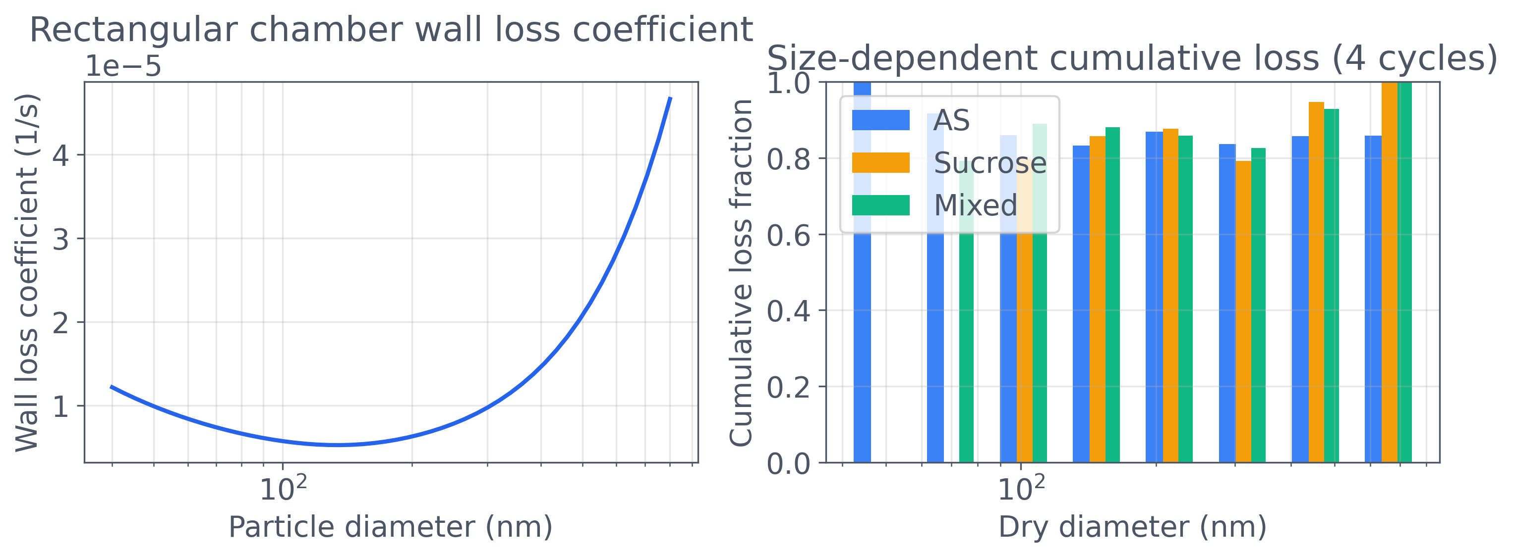
Use the gallery to ask four different questions
Section titled “Use the gallery to ask four different questions”The panels compare surviving-particle mean diameter, its peak and final values, initial/final dry mass and inferred dry deposition, and final bulk water fraction. Peak mean diameter is not the largest individual droplet. Dry inventory can decrease while wet diameter and wet mass increase. Read each diagnostic’s weighting rather than treating all bars as alternative measures of growth.
Python · section 18
# Panel A: mean diameter overlays (reuse prior calculations)panel_times = [times_as, times_sucrose, times_mixed]panel_means = [mean_diam_as, mean_diam_sucrose, mean_diam_mixed]panel_labels = ["AS", "Sucrose", "Mixed"]panel_colors = [    TAILWIND["blue"]["500"],    TAILWIND["amber"]["500"],    TAILWIND["emerald"]["500"],]
# Panel B: peak/mean diameter per scenariopeak_diams = [np.max(md) * 1e6 for md in panel_means]final_means = [md[-1] * 1e6 for md in panel_means]

# Panel C: mass balance (initial vs final vs loss)def total_mass(history):    masses0 = history[0]["masses"]    massesf = history[-1]["masses"]    init = masses0[:, :-1].sum()    final = massesf[:, :-1].sum()    return init, final, max(init - final, 0)

mass_init = []mass_final = []mass_loss = []for hist in [history_as, history_sucrose, history_mixed]:    init, final, loss = total_mass(hist)    mass_init.append(init)    mass_final.append(final)    mass_loss.append(loss)

# Panel D: final water mass fractiondef water_fraction(history, water_index):    masses = history[-1]["masses"]    total = masses.sum()    water = masses[:, water_index].sum()    return water / total if total > 0 else 0

water_fracs = [    water_fraction(history_as, water_index=1),    water_fraction(history_sucrose, water_index=1),    water_fraction(history_mixed, water_index=2),]
fig, axes = plt.subplots(2, 2, figsize=(10, 8))
# Aaxes[0, 0].set_title("Mean diameter over 4 cycles")for t, md, label, color in zip(    panel_times, panel_means, panel_labels, panel_colors):    axes[0, 0].plot(t / 60, md * 1e6, label=label, color=color, linewidth=2)axes[0, 0].set_xlabel("Time (minutes)")axes[0, 0].set_ylabel("Mean diameter (um)")axes[0, 0].legend()axes[0, 0].grid(alpha=0.3)
# Bxpos = np.arange(len(panel_labels))axes[0, 1].bar(    xpos - 0.15,    peak_diams,    width=0.3,    label="Peak",    color=TAILWIND["indigo"]["500"],)axes[0, 1].bar(    xpos + 0.15,    final_means,    width=0.3,    label="Final",    color=TAILWIND["gray"]["500"],)axes[0, 1].set_xticks(xpos)axes[0, 1].set_xticklabels(panel_labels)axes[0, 1].set_ylabel("Diameter (um)")axes[0, 1].set_title("Peak vs final mean diameter")axes[0, 1].legend()
# Cwidth = 0.25axes[1, 0].bar(    xpos - width,    mass_init,    width,    label="Initial",    color=TAILWIND["gray"]["400"],)axes[1, 0].bar(    xpos, mass_final, width, label="Final", color=TAILWIND["emerald"]["500"])axes[1, 0].bar(    xpos + width,    mass_loss,    width,    label="Dry wall deposition",    color=TAILWIND["rose"]["400"],)axes[1, 0].set_xticks(xpos)axes[1, 0].set_xticklabels(panel_labels)axes[1, 0].set_ylabel("Dry material mass (kg)")axes[1, 0].set_title("Dry inventory after 4 cycles")axes[1, 0].legend()
# Daxes[1, 1].bar(panel_labels, water_fracs, color=panel_colors)axes[1, 1].set_ylabel("Water / total mass")axes[1, 1].set_ylim(0, 1)axes[1, 1].set_title("Final water mass fraction")
plt.tight_layout()plt.show()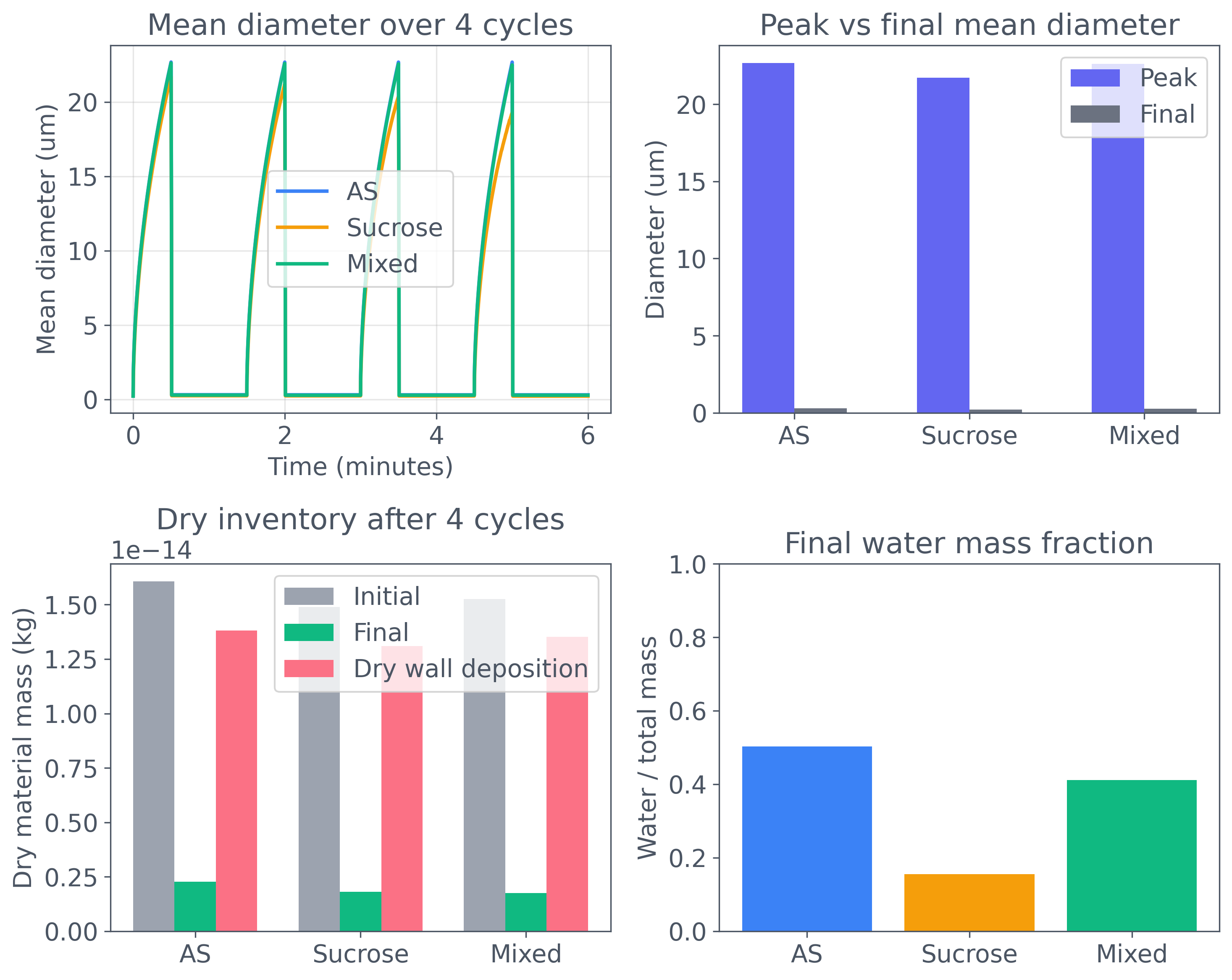
Contrast bulk water fraction with the earlier particle average
Section titled “Contrast bulk water fraction with the earlier particle average”Here each curve is total particle water divided by total particle mass. Larger wet particles therefore contribute more strongly than to the earlier equal-particle mean. Comparing the two statistics can reveal a heterogeneous population, but neither is a direct measure of wall deposition or critical supersaturation.
Python · section 19
def water_fraction_series(history, water_index):    times = []    fractions = []    for record in history:        masses = record["masses"]        total = masses.sum()        water = masses[:, water_index].sum()        fractions.append(water / total if total > 0 else 0)        times.append(record["time"])    return np.array(times), np.array(fractions)

wf_times = []wf_fracs = []for hist, widx in [    (history_as, 1),    (history_sucrose, 1),    (history_mixed, 2),]:    t_vals, f_vals = water_fraction_series(hist, widx)    wf_times.append(t_vals)    wf_fracs.append(f_vals)
cycle_marks = np.arange(0, n_cycles * cycle_duration + 1, cycle_duration)
plt.figure(figsize=(8, 4))for t_vals, f_vals, label, color in zip(    wf_times, wf_fracs, panel_labels, panel_colors):    plt.plot(t_vals / 60, f_vals, label=label, color=color, linewidth=2)for cm in cycle_marks:    plt.axvline(        cm / 60, color=TAILWIND["gray"]["300"], linestyle="--", linewidth=0.8    )plt.ylim(0, 1)plt.xlabel("Time (minutes)")plt.ylabel("Water mass fraction")plt.title("Water mass fraction evolution across cycles")plt.legend(loc="best")plt.tight_layout()plt.show()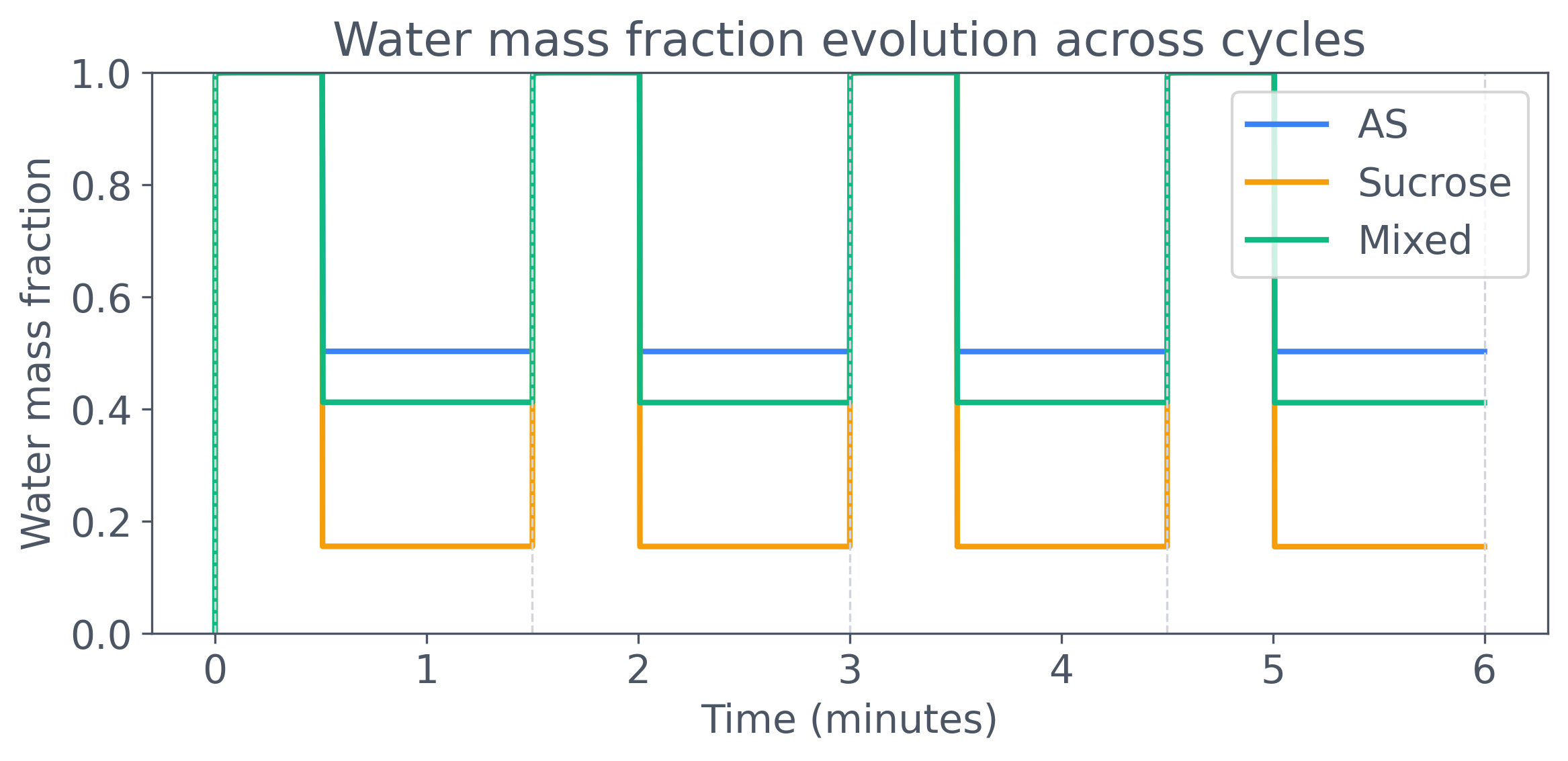
What the combined diagnostics establish
Section titled “What the combined diagnostics establish”Repeated vapor resets exchange water with surviving seeds while wall loss removes dry material. Tracking both species mass and particle identity separates those effects better than a size curve alone. In the refreshed realization, final dry-mass retention is about 14.1%, 12.1%, and 11.5% for sulfate, sucrose, and mixed seeds, respectively. The first-event check records 0.1 s for both pure compositions and therefore does not resolve an ordering between them. The adaptive ROS3 trajectories have smooth dry phases at the saved 0.1 s observation spacing, replacing the previous fixed-step oscillations. This does not establish convergence of the outer wall-loss schedule or accuracy between observations. Composition changes the activity model, but these separately sampled scenarios do not isolate a universal κ ordering or demonstrate competition between external sulfate and sucrose modes.
Design the next chamber comparison
Section titled “Design the next chamber comparison”For a research study, refine outer dt and condensation tolerances separately, keeping physical humid/dry durations fixed. Compare full size trajectories, dry retention, and the explicitly chosen activation diagnostic across independent random seeds. Then pair the initial radii across compositions to separate material effects from sample variability.
Measured humidity histories and chamber loss behavior would be needed to test the forcing and removal model. If dilution is added, use a process that updates the appropriate gas and particle inventories and account for its external flux; the unused reference coefficient in this example is not such a process.
Explore this topic: Chamber experiments · Condensation and evaporation · Wall loss and dilution