

Charged aerosols and ions across sixteen humid environments
Download Python script · Download script with helper and data files (.zip)
Charged aerosols and ions across sixteen environments
Section titled “Charged aerosols and ions across sixteen environments”How can we distinguish humidity-driven size growth from changes caused by particle collisions and ion attachment? This controlled factorial study compares size, number, and charge diagnostics across temperature, pressure, and initial humidity. It illustrates how several observables can separate mechanisms that a size spectrum alone cannot identify.
Use the condensation and prepared GPU guide as prerequisites. The intended outcome is to read these diagnostics together and design a controlled follow-up, rather than infer atmospheric rates from the example.
This CUDA example starts with 2,621,440 active resolved particles: 16 conditions × 1,024 independent boxes × (128 aerosols + 16 positive + 16 negative ions). All boxes remain resident together. Each particle has its own material masses and integer charge; its initial multiplicity is one. Boxes are well mixed, with no positions, electric fields or exchange between boxes.
The factorial grid contains temperatures of 278.15 and 298.15 K, pressures of 70,000 and 101,325 Pa, and initial relative humidities of 40, 60, 80 and 90%. These are controlled environments, not an altitude trajectory. Each condition starts with the same sampled particle population. The box volume keeps initial aerosol number concentration at 5 × 10¹³ m⁻³, an illustrative dense aerosol. All physical parameters here are demonstration assumptions.
Each step injects ion pairs, then applies water condensation/evaporation, followed by charge-dependent Brownian coagulation and ion collisions. A captured schedule advances 3,000 steps of 1 µs, totaling 3 ms. This resolves fast water-growth transients while making comparatively rare collisions visible across a large population. It is not a long-term atmospheric evolution or a CPU/GPU speed comparison.
Python · section 1
"""Run a manually refreshed two-million-particle charged CUDA sweep."""
import matplotlib.pyplot as pltimport numpy as npfrom scripts.gpu_studies.environment_sweep import (    EnvironmentSweep,    run_environment_sweep,)from scripts.gpu_studies.population_figures import (    describe_population,    ion_figures,    population_figures,)
Physical model and limitations
Section titled “Physical model and limitations”Each box starts with 16 ions of each sign (6.25 × 10¹² m⁻³ each). A source supplies 10¹⁴ ion pairs m⁻³ s⁻¹. This dense laboratory-style population is chosen to expose millisecond dynamics, not to represent ambient ion levels. Ion diameter is 0.5 nm; positive/negative masses are 150/90 u. Reference mobilities are illustrative 1.4/1.9 × 10⁻⁴ m² V⁻¹ s⁻¹ at 298.15 K, 1 atm, scaled as sqrt(T/298.15) × 101325/P. Ion friction is e/mobility. The Coulomb transition approximation omits image forces, trapping, hydration and ion chemistry. The explicitly fixed recombination coefficient is 1.7 × 10⁻¹² m³ s⁻¹; its T/P dependence is not modeled. Neutral products are exported every ten steps into a conserved mass ledger. Free ions and neutral products do not take up water; ion material remains nonvolatile.
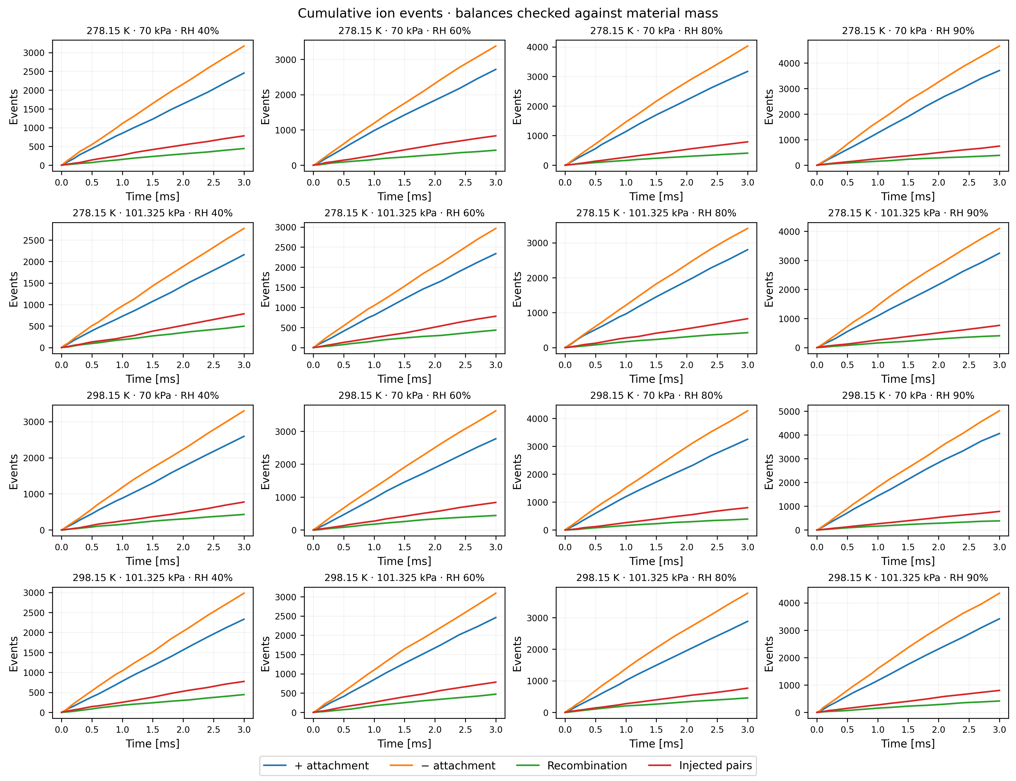
The aerosol spectra and merger plots exclude free ions and neutral products. Separate ion plots distinguish attachment, recombination and source events.
Dry radii follow a clipped lognormal distribution: geometric mean 35 nm, geometric standard deviation 1.6, bounds 15–150 nm. Dry density is 1,400 kg m⁻³. Initial water volume is 20% of dry volume. Water density is 1,000 kg m⁻³, surface tension 0.072 N m⁻¹ and accommodation coefficient one. The κ-water activity model uses illustrative dry κ = 0.3, with Kelvin curvature and Buck saturation vapor pressure. Every four initial particles carry charges −1, 0, 0, +1 elementary charges. Collisions add charge and all material masses. Explicit ions attach, transfer charge and recombine.
Vapor diffusivity is held at 2 × 10⁻⁵ m² s⁻¹ across conditions. The prepared interface accepts a species constant, not a per-box diffusion law. Thus this is a controlled transport approximation, not a complete prediction of temperature/pressure dependence. The supported formulas still use each box’s temperature and pressure. Temperature is prescribed; latent heat does not change it. Water vapor is finite and unreplenished, so the specified RH is initial RH, not a humidity controller.
The charged hard-sphere model uses Coulomb-modified Brownian collision rates. No empirical ion-attachment fit is extrapolated to these conditions. The Lucky Few example retains LF2013 at its fixed reference conditions. This study selects the separate mobility model.
Python · section 2
def simulate():    """Run the complete CUDA study and return compact numerical summaries."""    report, final = run_environment_sweep(EnvironmentSweep(ions=True))    del final    return report

def plot_results(report):    """Render saved observations without advancing the simulation."""    history = report["history"]    grid = np.array(report["conditions"])    time_ms = np.array([row["time"] for row in history]) * 1000    water = np.array([row["water_mass"] for row in history])    counts = np.array([row["count"] for row in history])    fig, axes = plt.subplots(2, 2, figsize=(10, 7), constrained_layout=True)    for panel, ax in enumerate(axes.flat):        for i in range(panel * 4, panel * 4 + 4):            ax.plot(                time_ms,                water[:, i] / water[0, i],                marker=".",                label=f"Initial RH {grid[i, 2]:.0%}",            )        temperature, pressure, _ = grid[panel * 4]        ax.set(            title=f"{temperature:.2f} K · {pressure / 1000:g} kPa",            xlabel="Time [ms]",            ylabel="Particle water mass / initial",        )        ax.legend(fontsize=8)        ax.grid(alpha=0.2)    fig.suptitle("Closed water uptake · 2,097,152 initial aerosols")
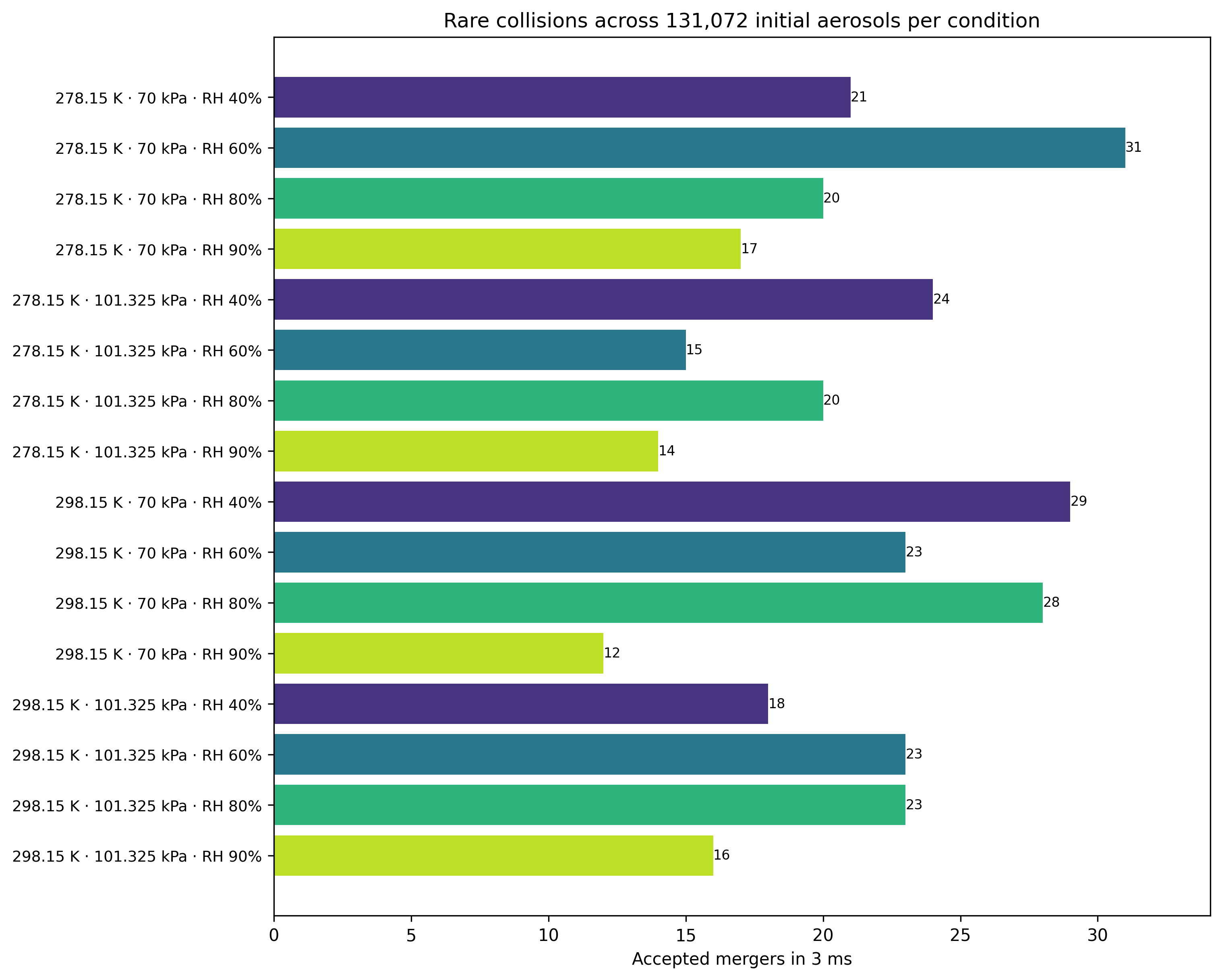
    fig, ax = plt.subplots(figsize=(10, 8), constrained_layout=True)    mergers = counts[0] - counts[-1]    colors = plt.get_cmap("viridis")(np.tile(np.linspace(0.15, 0.9, 4), 4))    ax.barh(np.arange(16), mergers, color=colors)    ax.set_yticks(        np.arange(16),        [f"{t:.2f} K · {p / 1000:g} kPa · RH {rh:.0%}" for t, p, rh in grid],    )    ax.tick_params(axis="y", labelsize=9)    ax.invert_yaxis()    ax.set_xlim(0, max(mergers.max() * 1.1, 1))    ax.set(        xlabel="Accepted mergers in 3 ms",        title="Rare collisions across 131,072 initial aerosols per condition",    )    ax.bar_label(ax.containers[0], fontsize=8)    print(f"Device: {report['device']}")    print(f"Initial active aerosols + ions: {report['initial_particles']:,}")    print(f"Final active aerosols: {counts[-1].sum():,}")    print(f"Total accepted mergers: {mergers.sum():,}")    print(        "Maximum per-box species-mass relative residual:",        f"{report['maximum_mass_relative_error']:.3e}",    )    print("Net charge is exactly conserved in every box at every diagnostic.")    print(f"Preparation/capture: {report['preparation_seconds']:.2f} s")    print(f"Synchronized stepping: {report['compute_seconds']:.2f} s")    print("T [K] | P [Pa] | initial RH | final mean RH | mergers")    for i, (temperature, pressure, rh) in enumerate(grid):        print(            f"{temperature:.2f} | {pressure:.0f} | {rh:.2f} | "            f"{history[-1]['rh'][i]:.6f} | {mergers[i]}"        )    print(        "Counts are one stochastic realization; differences are not significance tests."    )    labels = [        f"{t:.2f} K · {p / 1000:g} kPa · RH {rh:.0%}" for t, p, rh in grid    ]    population_figures(report, labels, time_scale=1000, time_unit="ms")    describe_population(report, labels)    ion_figures(report, labels)    return report

def run_example():    """Simulate once, then render the resulting numerical summaries."""    return plot_results(simulate())
Interpret the dynamics
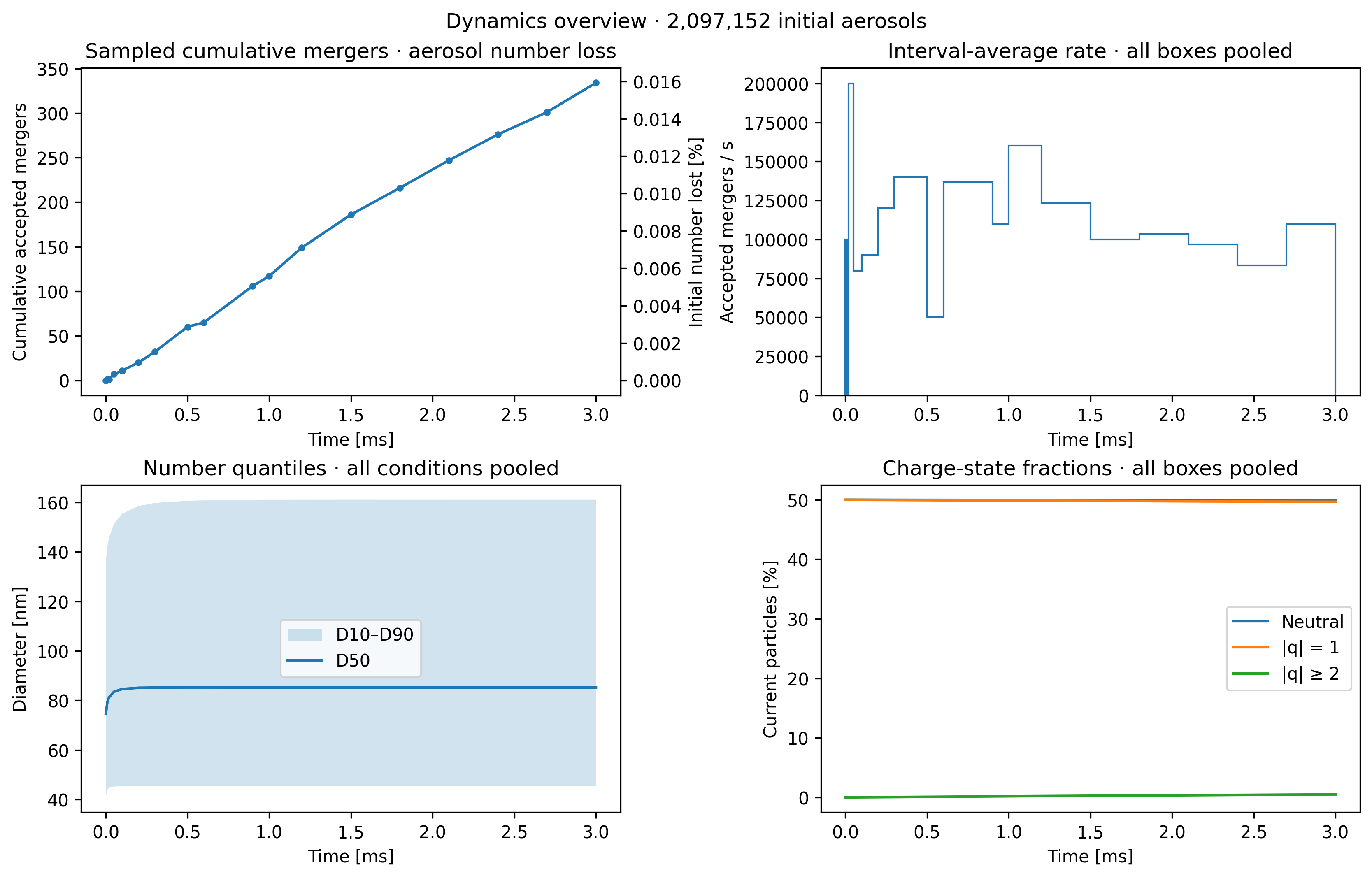
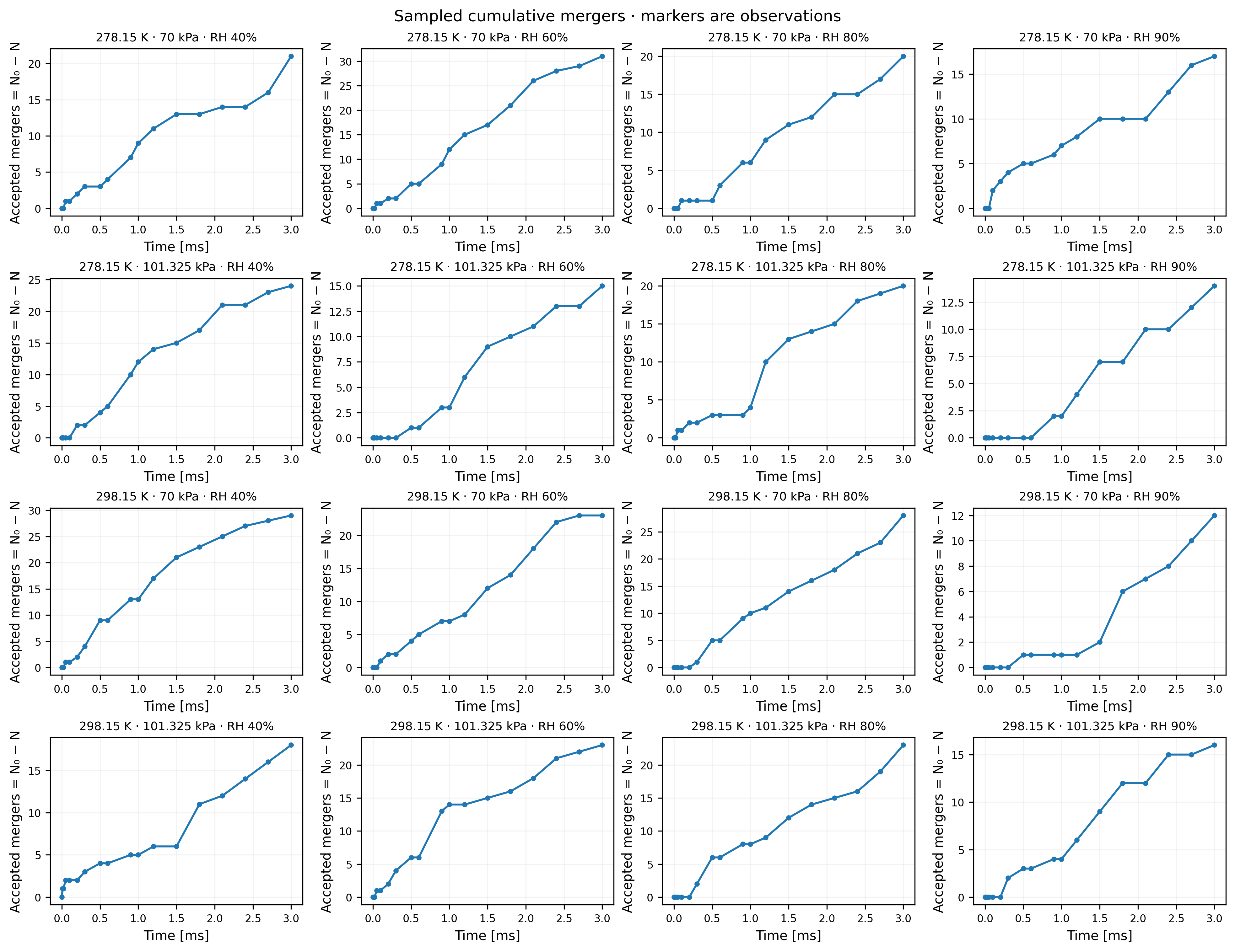
Section titled “Interpret the dynamics”The overview separates bulk size growth from the much rarer mergers. Water uptake changes particle diameter without changing particle number. Coagulation reduces number, moves dry and wet material into larger particles, and combines charges. Thus number lost equals accepted mergers here; it is not material lost from the box. There are no deposition or dilution sinks.
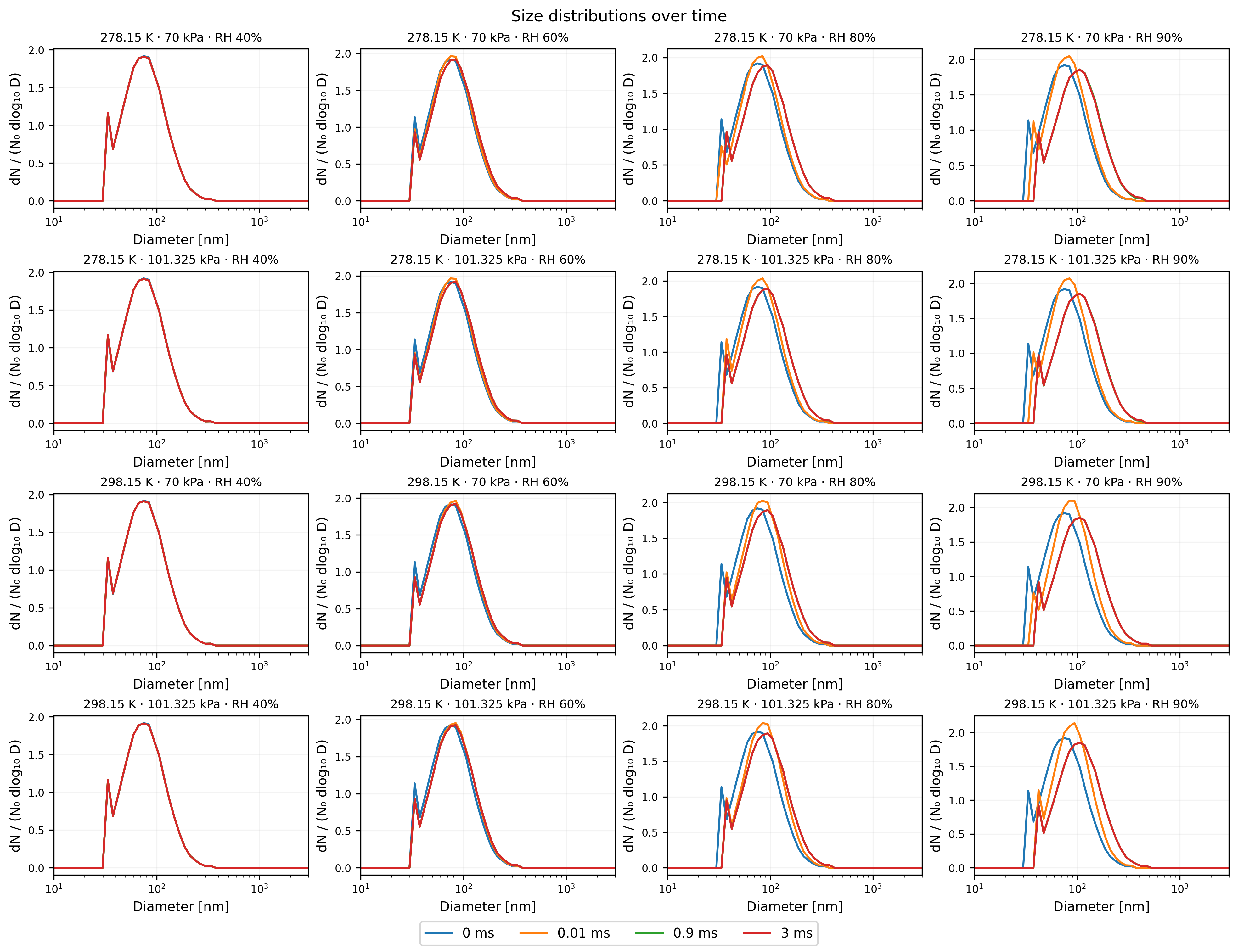
Each size-spectrum panel follows one environment. The ordinate is dN/(N₀ dlog₁₀D), with volume-equivalent diameter D. Integrating over log₁₀D yields the fraction of initial particles remaining, so normalization does not hide coagulation loss. Early diagnostic times resolve rapid water uptake; later curves show whether it is approaching a plateau.
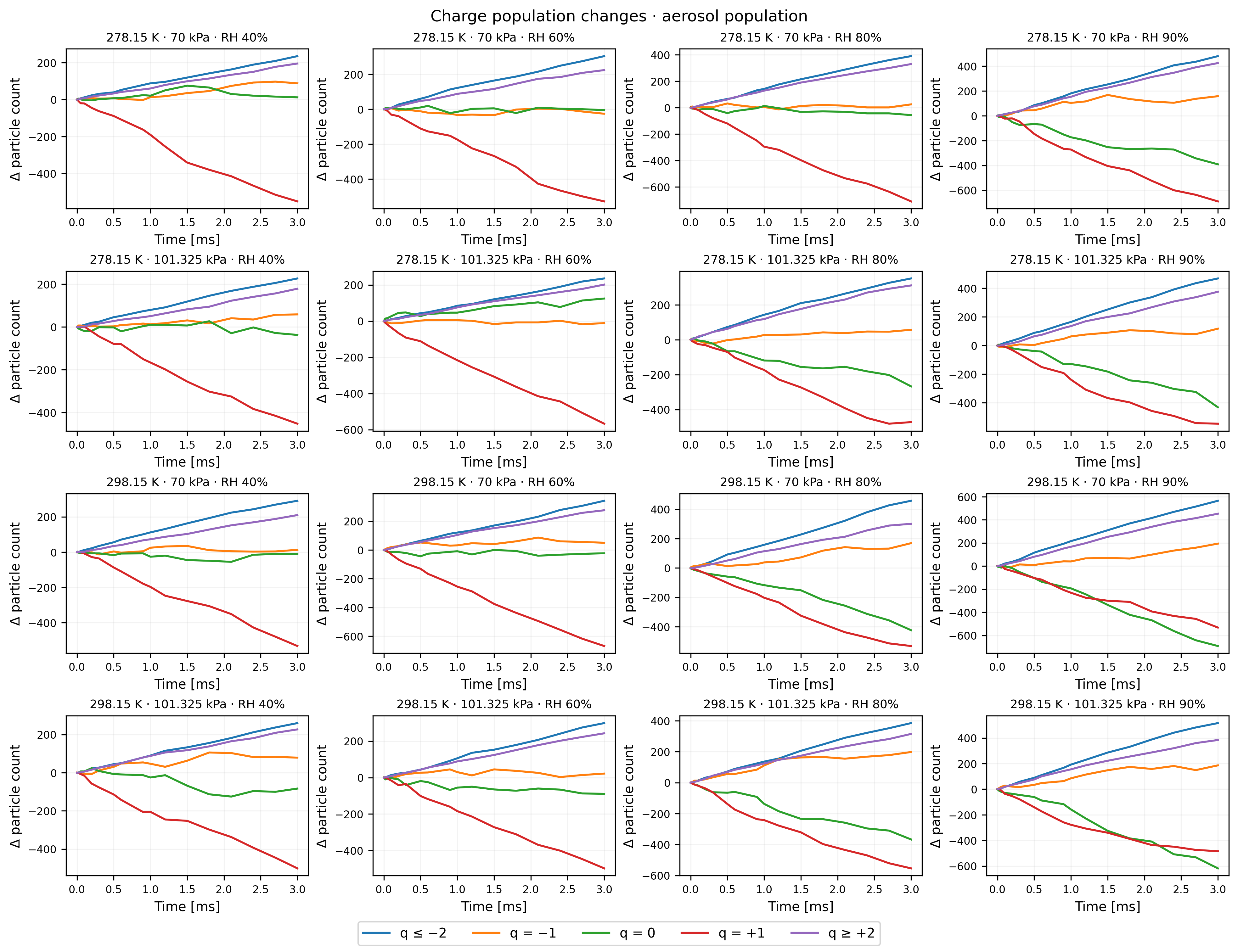
The charge overview gives fractions of the current population; the detailed panels instead show absolute changes in each charge class. The latter make rare neutralization and multiply charged particles visible even when the bulk fractions appear flat. Aerosol charge can change through attachment; total aerosol-plus-ion charge is conserved exactly.
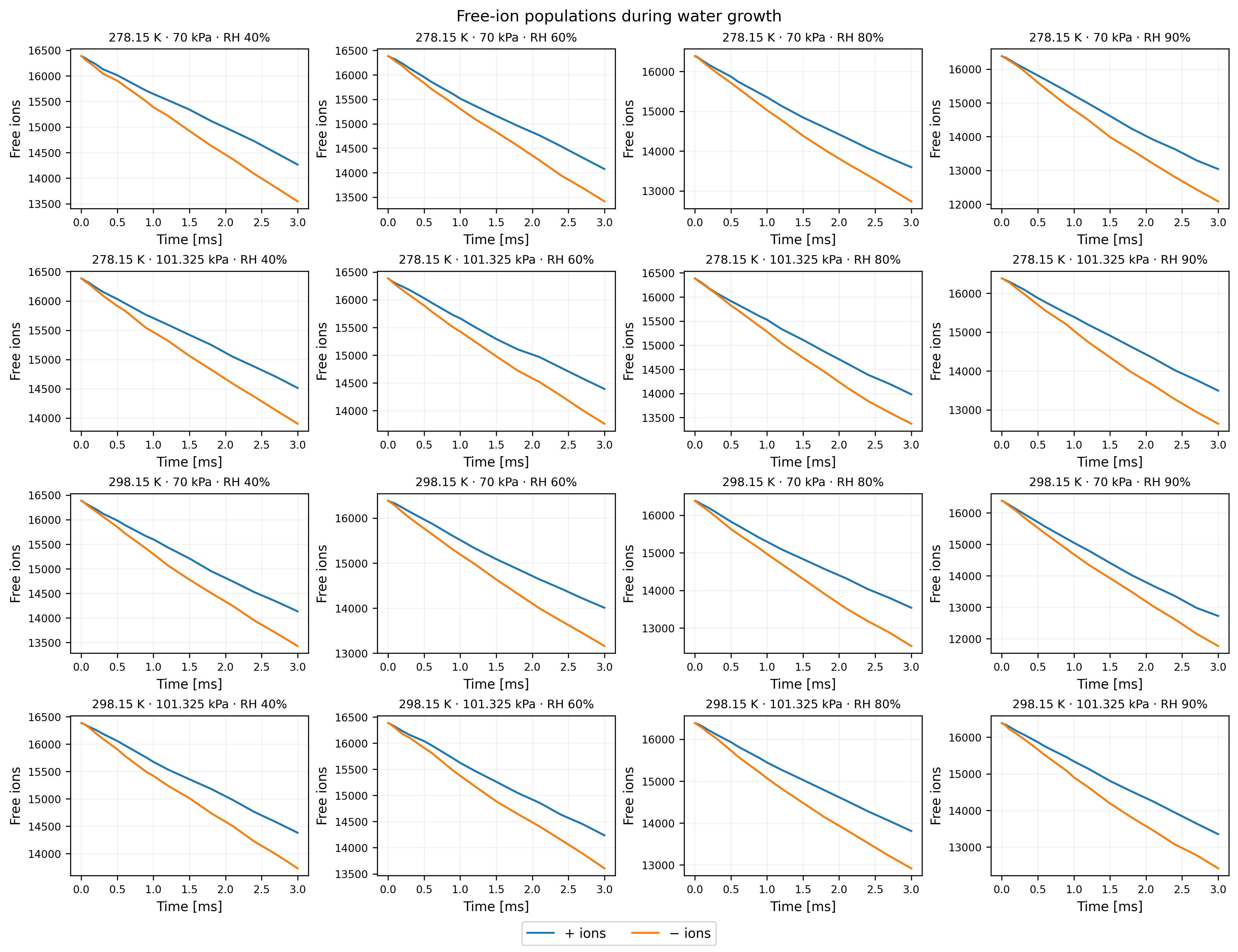
Read the ion histories alongside the charge panels. Attachment removes a free ion and transfers its charge to an aerosol; recombination removes one free ion of each sign and makes a neutral product. The source replenishes both signs equally. Different positive and negative attachment totals can therefore change aerosol net charge while the complete box stays neutral. The illustrative negative-ion mobility is larger than the positive value, but evolving aerosol charge and size also affect attachment. The plots report the combined response, not a measurement of either mobility alone.
Collision-rate values are averages over diagnostic intervals, not instantaneous rates or exact collision times. Small event counts create visible fluctuations. The bars retain ascending temperature, pressure and initial-humidity order, rather than sorting by the noisy outcomes. The printed interpretation reports measured size and count changes and identifies observed extrema without treating their ranking as a significance test.
At higher RH, this model supplies a larger water reservoir and equilibrium water content. Read the early rise and later plateau together: extending the duration can add collisions after most water growth has already occurred. Constant diffusivity and surface tension remain approximations. A dry altitude and high-pressure scan separately explores the much wider temperature/pressure domain without extrapolating this liquid-water treatment into the mesopause.
Numerical evidence and limits
Section titled “Numerical evidence and limits”The water curves distinguish evaporation, uptake and finite-time response. Each bar counts actual accepted mergers, inferred from the loss of resolved aerosols in this system. Each condition contains 1,024 independent boxes, but the bars are single-realization totals, without confidence intervals. They do not establish a statistically resolved environmental effect or charge enhancement relative to a neutral control.
Every diagnostic checks water gas + particle water, conserved dry material and exact net charge in each individual box. Mass tolerance is 2 × 10⁻¹¹ relative. Final masses must be finite and nonnegative. Separate small CUDA tests halve the water-growth timestep (1% particle mass, 0.1% vapor tolerances), compare CPU/CUDA condensation, and check κ-Köhler equilibrium against an independently written expression. Those tests qualify water integration; they do not establish stochastic convergence of the collision counts. The 3 ms endpoint need not be equilibrium for every particle.
Preparation and synchronized stepping timings exclude Python construction,
diagnostic reductions, state download and plotting. The downloadable ZIP
includes the helper; run python example.py in a compatible CUDA environment.
The full manual refresh can take hours and is not executed by routine CI.
References
Section titled “References”- Petters and Kreidenweis (2007): κ representation of water activity and hygroscopic growth. The selected κ value here is illustrative, not assigned to a measured material.
- Gopalakrishnan and Hogan (2012): hard-sphere transition-regime fit and charged collision scaling.
- The prepared execution guide documents resident ownership, CUDA capture and supported process contracts.
Python · section 3
if __name__ == "__main__": run_example()Explicit cuda invocation
result = run_example()Device: NVIDIA GeForce RTX 5060
Initial active aerosols + ions: 2,621,440
Final active aerosols: 2,096,818
Total accepted mergers: 334
Maximum per-box species-mass relative residual: 8.593e-14
Net charge is exactly conserved in every box at every diagnostic.
Preparation/capture: 2.07 s
Synchronized stepping: 6034.55 s
T [K] | P [Pa] | initial RH | final mean RH | mergers
278.15 | 70000 | 0.40 | 0.400020 | 21
278.15 | 70000 | 0.60 | 0.599183 | 31
278.15 | 70000 | 0.80 | 0.796821 | 20
278.15 | 70000 | 0.90 | 0.892833 | 17
278.15 | 101325 | 0.40 | 0.400020 | 24
278.15 | 101325 | 0.60 | 0.599183 | 15
278.15 | 101325 | 0.80 | 0.796821 | 20
278.15 | 101325 | 0.90 | 0.892820 | 14
298.15 | 70000 | 0.40 | 0.400006 | 29
298.15 | 70000 | 0.60 | 0.599757 | 23
298.15 | 70000 | 0.80 | 0.799041 | 28
298.15 | 70000 | 0.90 | 0.897735 | 12
298.15 | 101325 | 0.40 | 0.400006 | 18
298.15 | 101325 | 0.60 | 0.599757 | 23
298.15 | 101325 | 0.80 | 0.799041 | 23
298.15 | 101325 | 0.90 | 0.897735 | 16
Counts are one stochastic realization; differences are not significance tests.
Over 0.003 s: 334 accepted mergers; 2,096,818 particles remain (0.01593% number loss).
Pooled number-median diameter changes from 74.453 to 85.209 nm.
Largest recorded merger count: 278.15 K · 70 kPa · RH 60% (31); smallest: 298.15 K · 70 kPa · RH 90% (12).
Condition | initial count | final count | mergers | final D50 [nm]
278.15 K · 70 kPa · RH 40% | 131072 | 131051 | 21 | 74.259
278.15 K · 70 kPa · RH 60% | 131072 | 131041 | 31 | 78.726
278.15 K · 70 kPa · RH 80% | 131072 | 131052 | 20 | 88.941
278.15 K · 70 kPa · RH 90% | 131072 | 131055 | 17 | 101.840
278.15 K · 101.325 kPa · RH 40% | 131072 | 131048 | 24 | 74.255
278.15 K · 101.325 kPa · RH 60% | 131072 | 131057 | 15 | 78.721
278.15 K · 101.325 kPa · RH 80% | 131072 | 131052 | 20 | 88.936
278.15 K · 101.325 kPa · RH 90% | 131072 | 131058 | 14 | 101.838
298.15 K · 70 kPa · RH 40% | 131072 | 131043 | 29 | 74.269
298.15 K · 70 kPa · RH 60% | 131072 | 131049 | 23 | 78.774
298.15 K · 70 kPa · RH 80% | 131072 | 131044 | 28 | 89.255
298.15 K · 70 kPa · RH 90% | 131072 | 131060 | 12 | 103.184
298.15 K · 101.325 kPa · RH 40% | 131072 | 131054 | 18 | 74.267
298.15 K · 101.325 kPa · RH 60% | 131072 | 131049 | 23 | 78.779
298.15 K · 101.325 kPa · RH 80% | 131072 | 131049 | 23 | 89.256
298.15 K · 101.325 kPa · RH 90% | 131072 | 131056 | 16 | 103.191
Maximum mass residual: 8.593e-14; net charge is exactly conserved in every box.
One fixed-seed realization: rankings and interval-rate fluctuations are descriptive, not significance tests.
Ion events, pooled: attachment_positive: 46,354; attachment_negative: 58,889; recombination: 6,861; injected_pairs: 12,625
Aerosol number falls only through aerosol-aerosol mergers. Attachment transfers ion charge and mass without removing an aerosol; recombination removes two free ions and creates one inert neutral product.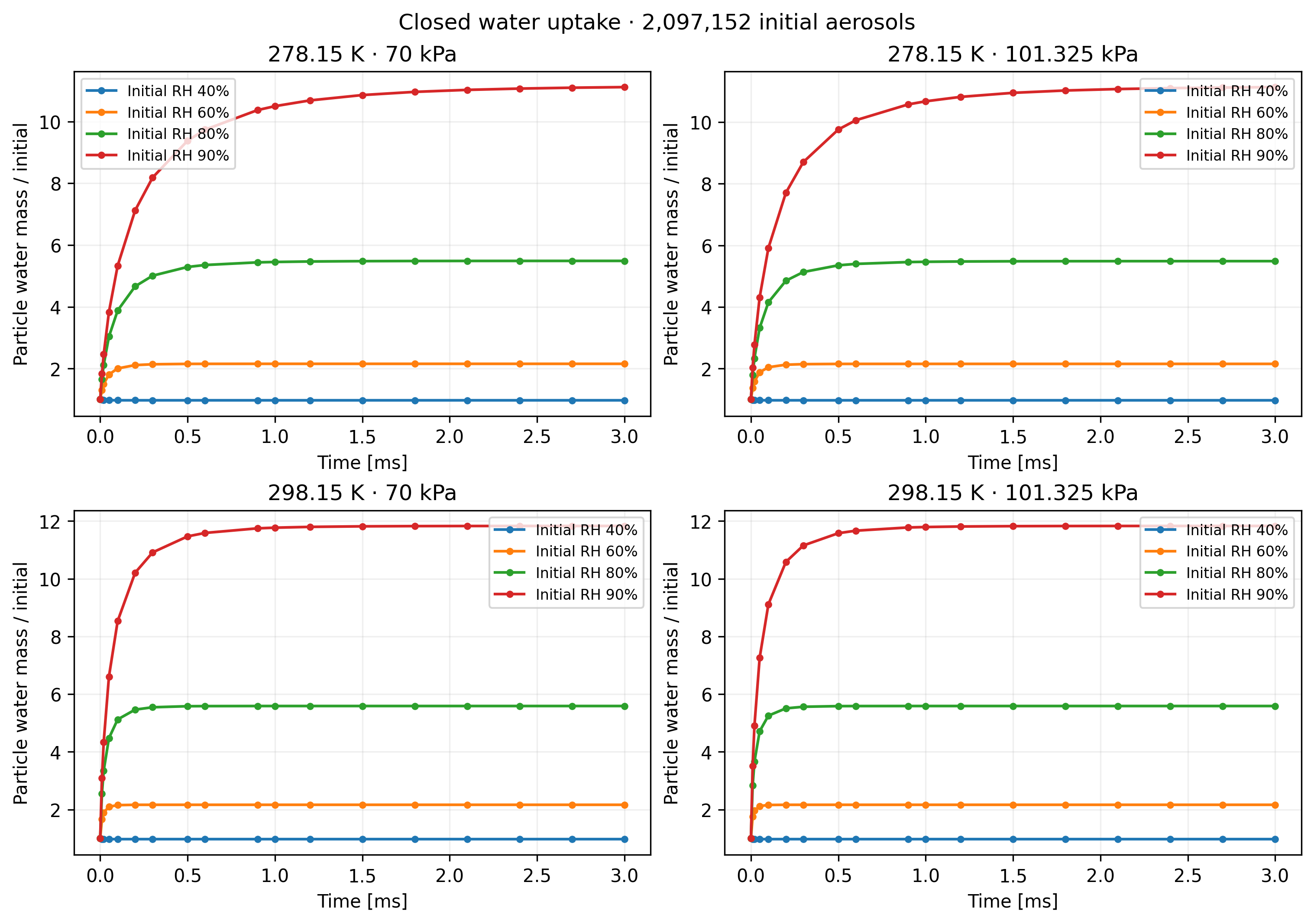
What the combined diagnostics tell us
Section titled “What the combined diagnostics tell us”Read the saved figures together: size change can occur through water exchange, while merger counts and aerosol-number loss diagnose collisions in this source/sink configuration. Aerosol charge alone is an incomplete inventory; the ion and neutral-product accounting supplies the rest of the interpretation. The interval-averaged rates and single-realization totals do not establish a statistically resolved ranking of environments.
To investigate charge enhancement in your own system, add a matched neutral control and repeat independent realizations. Compare merger counts with uncertainty estimates while checking material and charge budgets. To investigate humidity effects, hold the other environmental settings fixed and distinguish initial RH from a continuously maintained humidity. These controls and repeats are proposed extensions, not additional evidence in the saved run.
The existing dry environment sweep explores a different environmental domain; it does not extend the liquid-water assumptions to the mesopause. Choose the applicable physical model before expanding a sweep.
Explore this topic: Atmospheric processes · GPU workflows · Charged particles and ions