

Compare activity rules along a composition path
Python · section 1
"""Explore mixing rules and activity calculations.
This example walks through mass-based, molar-based, and volume-basedmixing rules, compares ideal activities, and demonstrates thekappa value parameterization to model non-ideal solution behavior. Eachsection builds the required data arrays, computes activities with thepublic ``par.particles`` helpers, and plots the results.
Example:    Run this example to generate activity plots for two- andthree-component systems under different mixing assumptions."""
'Explore mixing rules and activity calculations.\n\nThis example walks through mass-based, molar-based, and volume-based\nmixing rules, compares ideal activities, and demonstrates the\nkappa value parameterization to model non-ideal solution behavior. Each\nsection builds the required data arrays, computes activities with the\npublic ``par.particles`` helpers, and plots the results.\n\nExample:\n Run this example to generate activity plots for two- and\nthree-component systems under different mixing assumptions.\n'Compare activity rules along a composition path
Section titled “Compare activity rules along a composition path”How much can an assumed mixing rule change the activity assigned to the same mixture? We follow binary and ternary composition paths, comparing mole-, volume-, and mass-fraction rules with a κ water-activity parameterization. This helps separate a change of composition coordinates from a change of thermodynamic model before coupling activity to condensation.
Every vertical axis is activity, not activity coefficient. In the molar
standard-state convention,
Python · section 2
# In Colab uncomment the following command to install particula:# Install from the repository root: `python -m pip install -e ".[extra]"`import matplotlib.pyplot as pltimport numpy as npimport particula as parDefine the path before interpreting the curves
Section titled “Define the path before interpreting the curves”Water mass increases from 0 to 100 relative units while component 2 remains at 30. In the ternary path, component 3 decreases from 150 to 10. The common mass scale cancels in these rules; total mass is not held constant. Densities are kg/m³ and molar masses are kg/mol.
All panels use water mole fraction on the horizontal axis, computed once from these same masses. The ternary curves therefore trace one changing composition path, not a full ternary phase diagram. Component 3’s relative abundance changes at the same time as water’s.
Python · section 3
masses_1 = np.linspace(0, 100, 1000)masses_2 = np.full_like(masses_1, 30)masses_3 = np.linspace(150, 10, 1000)
density_1 = 1000  # kg/m^3density_2 = 2000  # kg/m^3density_3 = 1500  # kg/m^3
molar_mass_1 = 18.01528e-3  # kg/molmolar_mass_2 = 200e-3  # kg/molmolar_mass_3 = 150e-3  # kg/mol
mass_2component = np.column_stack((masses_1, masses_2))mass_3component = np.column_stack((masses_1, masses_2, masses_3))
density_2component = np.array([density_1, density_2])density_3component = np.array([density_1, density_2, density_3])
# get mole fractionsmole_fractions_2component = par.particles.get_mole_fraction_from_mass(    mass_2component, molar_masses=np.array([molar_mass_1, molar_mass_2]))mole_fractions_3component = par.particles.get_mole_fraction_from_mass(    mass_3component,    molar_masses=np.array([molar_mass_1, molar_mass_2, molar_mass_3]),)
Use mole fractions as the reference
Section titled “Use mole fractions as the reference”Ideal molar activity equals mole fraction. Water’s curve therefore lies on
Python · section 4
activity_2component_molar = par.particles.get_ideal_activity_molar(    mass_concentration=mass_2component,    molar_mass=np.array([molar_mass_1, molar_mass_2]),)

activity_3component_molar = par.particles.get_ideal_activity_molar(    mass_concentration=mass_3component,    molar_mass=np.array([molar_mass_1, molar_mass_2, molar_mass_3]),)

# Create the figure and axis objectsfig, ax = plt.subplots(2, 1, figsize=(5, 8))
# Plot each component in the 2-component system with separate colorsax[0].plot(    mole_fractions_2component[:, 0],    activity_2component_molar[:, 0],    color="blue",    label="Water (1)",)ax[0].plot(    mole_fractions_2component[:, 0],    activity_2component_molar[:, 1],    color="green",    label="Component 2",)ax[0].set_xlabel("Water Mole Fraction")ax[0].set_ylabel("Activity")ax[0].set_title("Binary molar-based activity")ax[0].legend()
# Plot the 3-component system without setting specific colorsax[1].plot(    mole_fractions_3component[:, 0],    activity_3component_molar[:, 0],    label="Water (1)",    color="blue",)ax[1].plot(    mole_fractions_3component[:, 0],    activity_3component_molar[:, 1],    label="Component 2",    color="green",)ax[1].plot(    mole_fractions_3component[:, 0],    activity_3component_molar[:, 2],    label="Component 3",    color="red",)ax[1].set_xlabel("Water Mole Fraction")ax[1].set_ylabel("Activity")ax[1].set_title("Ternary molar-based activity")ax[1].legend()
# Display the plotplt.tight_layout()plt.show()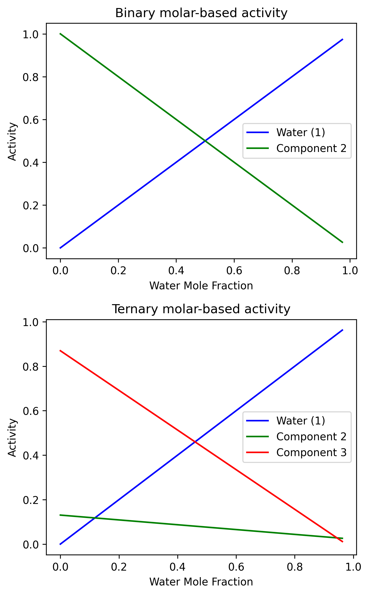
Weight by liquid volume
Section titled “Weight by liquid volume”The volume rule normalizes
Python · section 5
# Volume activityactivity_2component_volume = par.particles.get_ideal_activity_volume(    mass_concentration=mass_2component,    density=density_2component,)
activity_3component_volume = par.particles.get_ideal_activity_volume(    mass_concentration=mass_3component,    density=density_3component,)
# Create the figure and axis objectsfig, ax = plt.subplots(2, 1, figsize=(5, 8))
# Plot each component in the 2-component system with separate colorsax[0].plot(    mole_fractions_2component[:, 0],    activity_2component_volume[:, 0],    color="blue",    label="Water (1)",)ax[0].plot(    mole_fractions_2component[:, 0],    activity_2component_volume[:, 1],    color="green",    label="Component 2",)ax[0].set_xlabel("Water Mole Fraction")ax[0].set_ylabel("Activity")ax[0].set_title("Binary volume-based activity")ax[0].legend()
# Plot the 3-component system without setting specific colorsax[1].plot(    mole_fractions_3component[:, 0],    activity_3component_volume[:, 0],    label="Water (1)",    color="blue",)ax[1].plot(    mole_fractions_3component[:, 0],    activity_3component_volume[:, 1],    label="Component 2",    color="green",)ax[1].plot(    mole_fractions_3component[:, 0],    activity_3component_volume[:, 2],    label="Component 3",    color="red",)ax[1].set_xlabel("Water Mole Fraction")ax[1].set_ylabel("Activity")ax[1].set_title("Ternary volume-based activity")ax[1].legend()
# Display the plotplt.tight_layout()plt.show()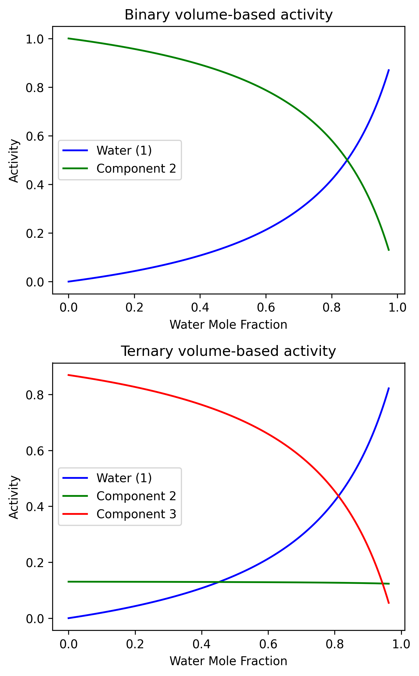
Weight by mass
Section titled “Weight by mass”The mass rule normalizes the input masses directly. Because water is much
lighter per molecule than either solute, its mass fraction is below its mole
fraction along these paths. The curved water trace against
Python · section 6
# Mass activityactivity_2component_mass = par.particles.get_ideal_activity_mass(    mass_concentration=mass_2component,)activity_3component_mass = par.particles.get_ideal_activity_mass(    mass_concentration=mass_3component,)
# Create the figure and axis objectsfig, ax = plt.subplots(2, 1, figsize=(5, 8))
# Plot each component in the 2-component system with separate colorsax[0].plot(    mole_fractions_2component[:, 0],    activity_2component_mass[:, 0],    color="blue",    label="Water (1)",    linewidth=4,    linestyle="--",)ax[0].plot(    mole_fractions_2component[:, 0],    activity_2component_mass[:, 1],    color="green",    label="Component 2",)ax[0].set_xlabel("Water Mole Fraction")ax[0].set_ylabel("Activity")ax[0].set_title("Binary mass-based activity")ax[0].legend()
# Plot the 3-component system without setting specific colorsax[1].plot(    mole_fractions_3component[:, 0],    activity_3component_mass[:, 0],    label="Water (1)",    color="blue",    linewidth=4,    linestyle="--",)ax[1].plot(    mole_fractions_3component[:, 0],    activity_3component_mass[:, 1],    label="Component 2",    color="green",    linewidth=3,)ax[1].plot(    mole_fractions_3component[:, 0],    activity_3component_mass[:, 2],    label="Component 3",    color="red",)ax[1].set_xlabel("Water Mole Fraction")ax[1].set_ylabel("Activity")ax[1].set_title("Ternary mass-based activity")ax[1].legend()
# Display the plotplt.tight_layout()plt.show()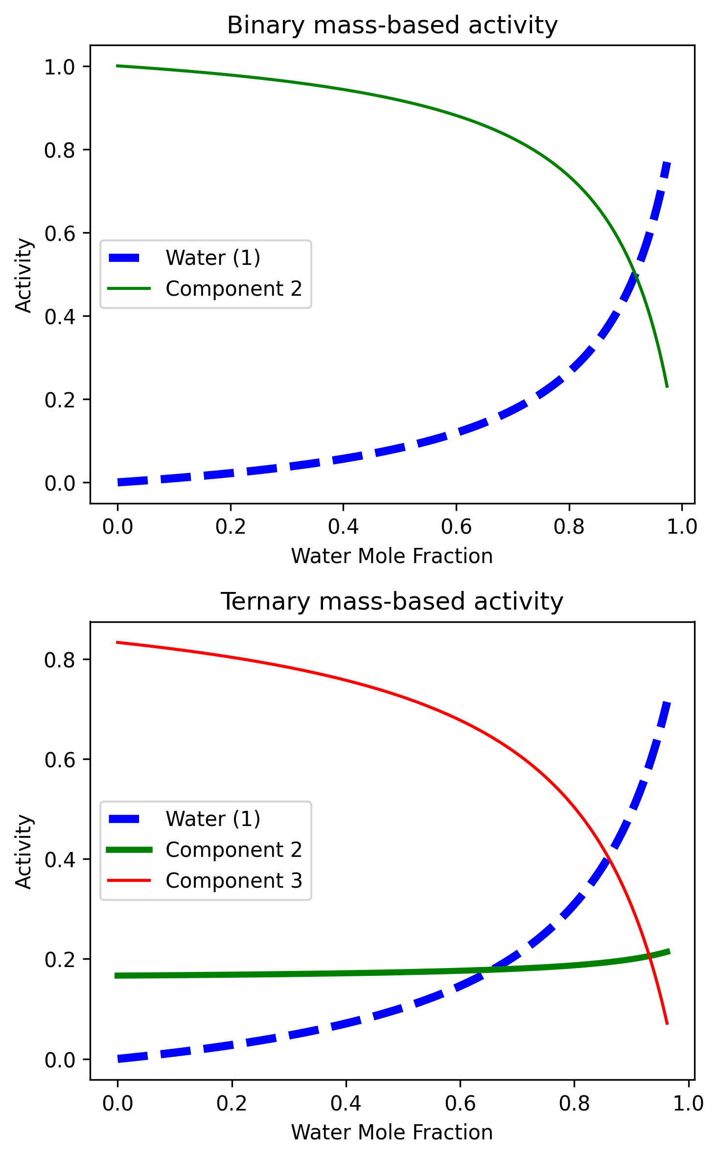
Change water’s rule with κ
Section titled “Change water’s rule with κ”The illustrative solutes have κ=0.6 and 1.2; the water lane’s κ is unused.
Water activity follows
The nonwater lanes retain ideal molar activities. Compare them with the first pair of panels to see that this model changes water’s rule without computing nonideal activity coefficients for every component. The parameterization follows Petters and Kreidenweis (2007); the particular solute parameters here are illustrative.
Python · section 7
# kappa activity
kappa_1 = 0.0  # kappa of waterkappa_2 = 0.6  # kappa of component 2kappa_3 = 1.2  # kappa of component 3
water_index = 0
activity_2component_kappa = par.particles.get_kappa_activity(    mass_concentration=mass_2component,    kappa=np.array([kappa_1, kappa_2]),    density=density_2component,    molar_mass=np.array([molar_mass_1, molar_mass_2]),    water_index=water_index,)activity_3component_kappa = par.particles.get_kappa_activity(    mass_concentration=mass_3component,    kappa=np.array([kappa_1, kappa_2, kappa_3]),    density=density_3component,    molar_mass=np.array([molar_mass_1, molar_mass_2, molar_mass_3]),    water_index=water_index,)
# Create the figure and axis objectsfig, ax = plt.subplots(2, 1, figsize=(5, 8))
# Plot each component in the 2-component system with separate colorsax[0].plot(    mole_fractions_2component[:, 0],    activity_2component_kappa[:, 0],    color="blue",    label="Water (1)",)ax[0].plot(    mole_fractions_2component[:, 0],    activity_2component_kappa[:, 1],    color="green",    label="Component 2",)ax[0].set_xlabel("Water Mole Fraction")ax[0].set_ylabel("Activity")ax[0].set_title("Binary κ activity")ax[0].legend()
# Plot the 3-component system without setting specific colorsax[1].plot(    mole_fractions_3component[:, 0],    activity_3component_kappa[:, 0],    label="Water (1)",    color="blue",)ax[1].plot(    mole_fractions_3component[:, 0],    activity_3component_kappa[:, 1],    label="Component 2",    color="green",)ax[1].plot(    mole_fractions_3component[:, 0],    activity_3component_kappa[:, 2],    label="Component 3",    color="red",)ax[1].set_xlabel("Water Mole Fraction")ax[1].set_ylabel("Activity")ax[1].set_title("Ternary κ activity")ax[1].legend()
# Display the plotplt.tight_layout()plt.show()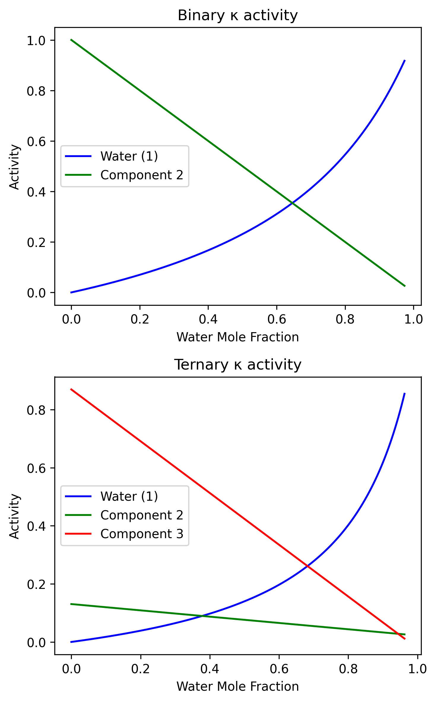
What survives a change of mixing rule?
Section titled “What survives a change of mixing rule?”The composition path and its mole-fraction coordinate stay fixed, while the predicted activities change. Thus interpreting a condensation calculation requires naming its activity approximation as well as its composition. Agreement at an endpoint or the fact that fractions sum to one does not choose the physically appropriate rule.
For a research comparison, hold the dry solute ratio fixed, vary only water,
and compare predicted
Explore this topic: Chemical activity