

Map charged collision rates with a factory
Python · section 1
"""Demonstrate the factory-based charged coagulation workflow with particula.
The tutorial constructs a charged particle size distribution, derives supportingtransport properties, obtains a charged strategy through CoagulationFactory, andvisualizes the resulting kernel on a log-log grid.
Examples:    >>> par.dynamics.CoagulationFactory().get_strategy(    ...     "charged",    ...     parameters={"distribution_type": "discrete",    ...                 "charged_kernel_strategy": par.dynamics.CoulombGatti2008KernelStrategy()},    ... )"""
'Demonstrate the factory-based charged coagulation workflow with particula.\n\nThe tutorial constructs a charged particle size distribution, derives supporting\ntransport properties, obtains a charged strategy through CoagulationFactory, and\nvisualizes the resulting kernel on a log-log grid.\n\nExamples:\n >>> par.dynamics.CoagulationFactory().get_strategy(\n ... "charged",\n ... parameters={"distribution_type": "discrete",\n ... "charged_kernel_strategy": par.dynamics.CoulombGatti2008KernelStrategy()},\n ... )\n'Map charged collision rates with a factory
Section titled “Map charged collision rates with a factory”Which size pairs can collide readily when their charges differ? This example constructs a two-particle collision-kernel matrix using the Coulomb Gatti 2008 strategy. It helps you connect a prescribed size–charge relation to pairwise rates before attempting a population simulation.
The companion construction uses the same physics through another configuration interface. Neither page evolves an aerosol or specifies how many particles occupy each size; a kernel in m³ s⁻¹ is not an event rate until it is combined with population abundance.
Python · section 2
import matplotlib.pyplot as pltimport numpy as npimport particula as par
plt.rcParams["figure.dpi"] = 110
Specify particle sizes without inventing a population
Section titled “Specify particle sizes without inventing a population”The 250 radius nodes span 1 nm–100 µm. Spherical mass uses density 1000 kg m⁻³. This broad grid explores kernel behavior; it is not a measured size distribution or a claim that one material model is applicable over every radius. No bin concentrations are supplied.
Python · section 3
radius_bins = np.logspace(start=-9, stop=-4, num=250) # m (1 nm to 100 μm)mass_bins = 4 / 3 * np.pi * radius_bins**3 * 1e3 # kg (ρ = 1000 kg/m³)n_bins = len(radius_bins)Prescribe a size–charge relation
Section titled “Prescribe a size–charge relation”The smallest third of nodes carries negative charge, varying from −10 to −1 in elementary-charge units. The remaining nodes carry positive charge from +1 to +500. The plotted discontinuity is imposed by this assignment, not predicted by charging dynamics. Fractional values are used as a parameter sweep; individual particle charges would be quantized.
Use this first plot to locate unlike-sign and like-sign regions in the later pair matrix. It does not represent a charge distribution at a given size or an ion-balance calculation.
Python · section 4
split_index = n_bins // 3neg_charges = -np.logspace(np.log10(10), np.log10(1), num=split_index)pos_charges = np.logspace(np.log10(1), np.log10(500), num=n_bins - split_index)charge_array = np.concatenate((neg_charges, pos_charges))
fig, ax = plt.subplots()ax.plot(radius_bins, charge_array, marker="o", linestyle="none")ax.set_xscale("log")ax.set_yscale("symlog", linthresh=1)ax.set_xlabel("Particle radius (m)")ax.set_ylabel("Particle charge (elementary charges)")ax.set_title("Particle Charge vs. Radius")ax.grid(True, which="both", ls="--")plt.show()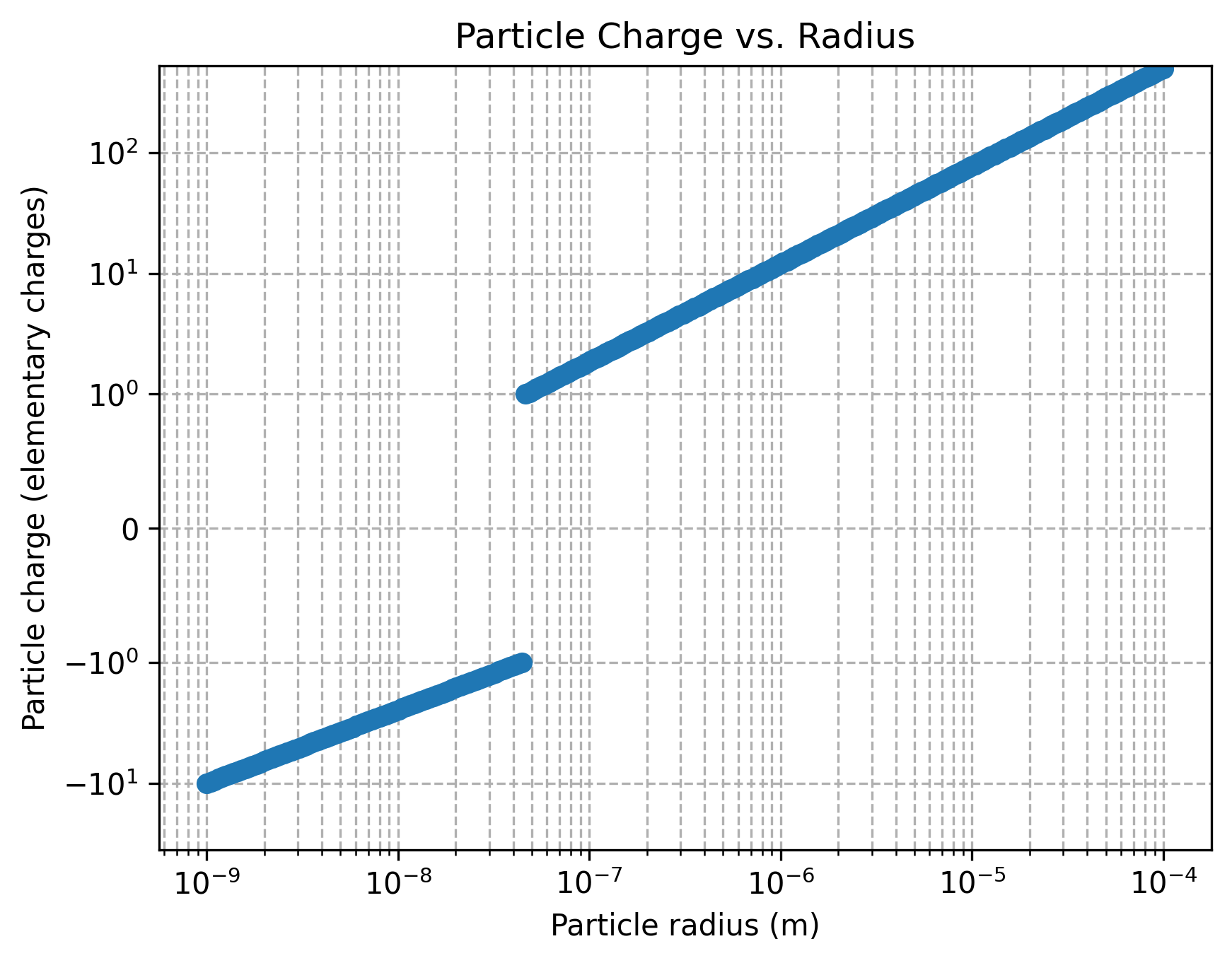
Connect electrostatics with transport
Section titled “Connect electrostatics with transport”At 298.15 K, the Coulomb ratio compares electrostatic interaction with thermal energy. Gas viscosity, mean free path, slip correction, and friction connect radius to transport; reduced mass and friction describe a pair. The diffusive Knudsen matrix then places each pair in the kernel’s transport regime.
These calculations use the gas helpers’ defaults where arguments are omitted. A pressure-sensitivity study must explicitly set and propagate the intended gas conditions rather than changing temperature alone.
Python · section 5
temperature = 298.15  # K
coulomb_potential_ratio: np.ndarray = np.asarray(    par.particles.get_coulomb_enhancement_ratio(        radius_bins, charge_array, temperature=temperature    ),    dtype=float,)dynamic_viscosity = par.gas.get_dynamic_viscosity(temperature=temperature)mol_free_path = par.gas.get_molecule_mean_free_path(    temperature=temperature, dynamic_viscosity=dynamic_viscosity)knudsen_number = par.particles.get_knudsen_number(    mean_free_path=mol_free_path, particle_radius=radius_bins)slip_correction = par.particles.get_cunningham_slip_correction(    knudsen_number=knudsen_number)friction_factor_value = par.particles.get_friction_factor(    particle_radius=radius_bins,    dynamic_viscosity=dynamic_viscosity,    slip_correction=slip_correction,)diffusive_knudsen_values: np.ndarray = np.asarray(    par.particles.get_diffusive_knudsen_number(        particle_radius=radius_bins,        particle_mass=mass_bins,        friction_factor=friction_factor_value,        coulomb_potential_ratio=coulomb_potential_ratio,        temperature=temperature,    ),    dtype=float,)
sum_of_radii = radius_bins[:, np.newaxis] + radius_bins[np.newaxis, :]reduced_mass = par.util.get_reduced_self_broadcast(mass_bins)reduced_friction_factor = par.util.get_reduced_self_broadcast(    friction_factor_value)
Select the physical kernel through configuration
Section titled “Select the physical kernel through configuration”The factory chooses the charged strategy from a parameter dictionary. The
selected Coulomb Gatti 2008 model then computes a dimensionless kernel and
restores its dimensions using pair geometry, mass, and friction. Selecting
discrete configures a strategy; this page calls its kernel model directly,
without advancing any distribution.
Python · section 6
factory = par.dynamics.CoagulationFactory()kernel_strategy = par.dynamics.CoulombGatti2008KernelStrategy()coagulation_strategy = factory.get_strategy(    "charged",    parameters={        "distribution_type": "discrete",        "charged_kernel_strategy": kernel_strategy,    },)
dimensionless_kernel = coagulation_strategy.kernel_strategy.dimensionless(    diffusive_knudsen=diffusive_knudsen_values,    coulomb_potential_ratio=coulomb_potential_ratio,)dimensional_kernel = coagulation_strategy.kernel_strategy.kernel(    dimensionless_kernel=dimensionless_kernel,    coulomb_potential_ratio=coulomb_potential_ratio,    sum_of_radii=sum_of_radii,    reduced_mass=reduced_mass,    reduced_friction_factor=reduced_friction_factor,)
particula/dynamics/coagulation/charged_dimensionless_kernel.py:203: RuntimeWarning: divide by zero encountered in divide
factored_term = (pi_sqrt * continuum * coulomb_potential_ratio * 1.22) / (
particula/dynamics/coagulation/charged_dimensionless_kernel.py:208: RuntimeWarning: invalid value encountered in multiply
term1 = continuum_limit * (1 - (1 + factored_term) * exponential_decay)
particula/dynamics/coagulation/charged_dimensionless_kernel.py:214: RuntimeWarning: divide by zero encountered in divide
+ (
particula/dynamics/coagulation/charged_dimensionless_kernel.py:210: RuntimeWarning: invalid value encountered in multiply
np.sqrt(8 * np.pi)Read the pair matrix and its numerical boundaries
Section titled “Read the pair matrix and its numerical boundaries”Each location refers to a pair of radii, with charges obtained from the first plot. The color is the base-10 logarithm of the kernel’s numerical value in m³ s⁻¹. Like-sign repulsion and unlike-sign attraction influence the structure, but transport and size also vary, so this matrix alone does not isolate the charge effect from those other dependencies.
The saved run emits divide-by-zero and invalid-operation warnings in intermediate expressions over this broad range. The final assertions require finite, nonnegative, symmetric kernel values. Exact zeros are masked on the logarithmic plot; blank regions must not be interpreted as a measured positive rate. Passing final-array checks does not validate an extreme parameter regime.
Python · section 7
assert np.all(np.isfinite(dimensional_kernel))assert np.all(dimensional_kernel >= 0)np.testing.assert_allclose( dimensional_kernel, dimensional_kernel.T, rtol=1e-12, atol=0)log_kernel = np.ma.log10(np.ma.masked_less_equal(dimensional_kernel, 0))fig, ax = plt.subplots()mesh = ax.pcolormesh(radius_bins, radius_bins, log_kernel, shading="auto")ax.set_xscale("log")ax.set_yscale("log")ax.set_xlabel("Particle radius r_i (m)")ax.set_ylabel("Particle radius r_j (m)")ax.set_title("Coulomb Gatti 2008 Coagulation Kernel (Factory)")fig.colorbar(mesh, ax=ax, label="log10(Kernel) (m³/s)")plt.show()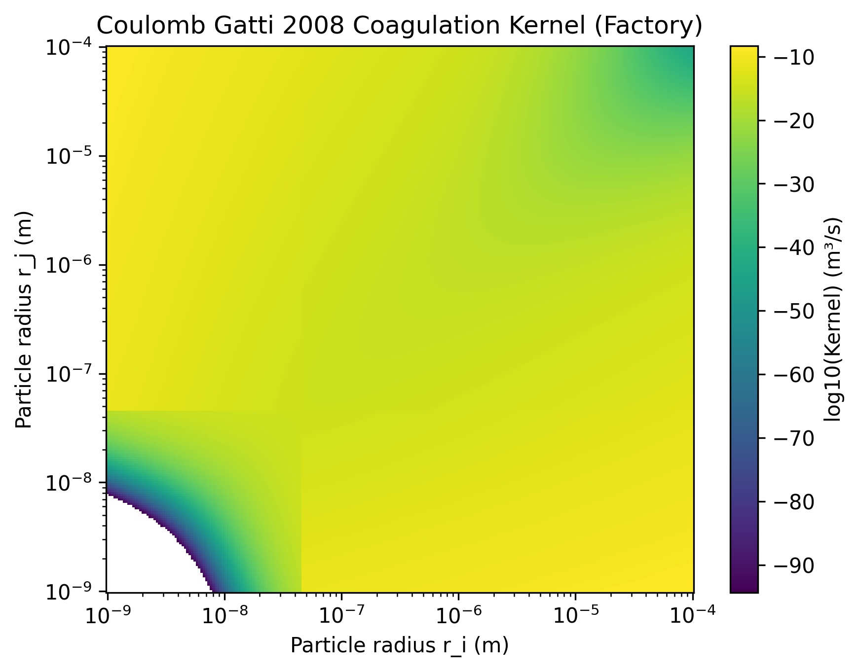
Turn the map into a charging experiment
Section titled “Turn the map into a charging experiment”The matrix identifies which prescribed pairs have larger or smaller modeled collision coefficients. It cannot predict a population lifetime without number concentrations, nor establish how the imposed charges arise.
To isolate a charging effect, repeat the kernel calculation at the same radii and gas conditions for neutral, same-sign, and opposite-sign assignments. Compare ratios only where the reference is finite and nonzero, inspect limiting behavior, and document the model’s applicable regime. Then use an independently specified size/charge population to compute collision rates. The Brownian time-evolution example provides a neutral population baseline; coupling charging dynamics would require additional physics and validation.
Explore this topic: Charged particles and ions